BASIC INFORMATION
This is the notes of the course “Provable Security”. The first few courses will be taught online. While subsequent courses are still unsettled.
I took this course last year, and I am pretty confident about my grasp of basic concepts like universal hash function, GL theorem, basic PRG, PRF constructions, etc. But contents like CRHF and PRP are still rather alien to me, so in this course I will review the previous contents and try to master the missing pieces. Also it is desireable to incopreate the previous notes and complete the notes altogegher.
| TEACHER | 郁昱,刘振 |
|---|---|
| LOCATION | 陈瑞球楼108 |
| CODE | C033728200203300M01 |
| ZOOM NUMBER | 284739677 |
| ZOOM CODE | 09333040 |
| LINK | https://zoom.com.cn/j/284739677 |
Homework
This section is dedicated to all homework and exercises throughout the lecture (along with their solutions of course).
18-19-2 Lecture 2
- Prove conditional LHL
- Non-existence of deterministic randomness extractor
- one-time message authentication code
- equivalence between min-entropy and collision entropy
For solutions please refer to Here.
18-19-2 Lecture 4
- Improving advantage in GL-theorem proof,i.e., difference between guessing game (exact preimage) and inverting game (any satisfying preimage).
- Exercies 6.1 6.2 6.4 6.6 from KL book
Answer can be found here.
19-20-2 Lecture 2
Existence of independent code here.
For an event \(E\), we use the indicator function
\[ I(E) = \begin{cases} 1 & E\\ 0 & \bar{E} \end{cases}\enspace. \]
Fix an \(i\), we bound the probability
\[ p = \Pr_{C}[\Pr_{r\leftarrow R_i^m}[Cr = 0] > \frac{1+\zeta}{2^n}]. \]
First we expand the inner probability expression
\[ p = \Pr_C[\frac{1}{\binom{m}{i}} (\sum_{r^{\prime}: |r^{\prime}| = i}I(Cr^{\prime} = 0)) > \frac{1+\zeta}{2^n}]. \]
And then we transform the form to facilitate Chebyshev’s Inequality. (It is easy to observe that \(\mathsf{E}_{C}[I(Cr=0)] = \frac{1}{2^n}\).)
\begin{align*} p &= \Pr_C[(\sum_{r^{\prime}: |r^{\prime}| = i}I(Cr^{\prime} = 0)) - \frac{\binom{m}{i}}{2^n} > \binom{m}{i} \frac{\zeta}{2^n}] \\ &\le \Pr_C[\left| (\sum_{r^{\prime}: |r^{\prime}| = i}I(Cr^{\prime} = 0)) - \frac{\binom{m}{i}}{2^n} \right| > \binom{m}{i} \frac{\zeta}{2^n}] \\ &\le \frac{\underset{C}{Var}{(\sum_{r^{\prime}: |r^{\prime}| = i}I(Cr^{\prime} = 0))}} {(\binom{m}{i} {\frac{\zeta}{2^n}})^2}\enspace. \end{align*}
Notice that for distinct \(r_1\) and \(r_2\), the random variable \(I(C r_1 = 0\) and \(I(C r_2 = 0\) are independent since \(I(C (r_1 - r_2)\) follows the same distribution as either of them. This means we can further expand the expression as
\[ p \le \frac{ \sum_{r^{\prime}: |r^{\prime}| = i}\underset{C}{Var}{(I(Cr^{\prime} = 0))}}{(\binom{m}{i} {\frac{\zeta}{2^n}})^2}\enspace. \]
Since once \(r\) is fixed, \(I(Cr = 0)\) follows the Bernoulli distribution with \(\mu = \frac{1}{2^n}\), we can further write the expression as
\begin{align*}~ p &\le \frac{ \binom{m}{i} \mu - \mu^2}{(\binom{m}{i} {\frac{\zeta}{2^n}})^2} \\ &\le \frac{2^n \binom{m}{i}^{-1}}{\zeta^2}\enspace. \end{align*}
Since \(i \le \frac{k}{2}\) and \(\binom{m}{i} \ge \binom{m}{k/2} \ge (\frac{m}{k/2})^{k/2}\), we have
\begin{align*} p &\le \frac{2^{n - \frac{k}{2} \log{\frac{2m}{k}}}}{\zeta^2} \\ &\le \frac{2^{n - \frac{k}{2} \log{\frac{m}{k}} + \frac{\log m}{2}}} {\zeta^2}\enspace. \end{align*}
Using a union bound on all possible values of \(i\), we conclude the proof of this lemma.
19-20-2 Lecture 5
PRG from LPN
Link: Lecture 5
Following usual LPN conventions, we define the LPN distribution \(LPN_{n,\mu}^m := (A, As+e)\), where \(A\leftarrow U_{m\times n}\), \(s\leftarrow U_n\), and \(e \leftarrow Ber_{\mu}^m\). The (\(n\), \(\mu\), \(m\))-DLPN assumption postulate that for any probablistic polynomial time distinguisher, the advantage of distinguishing \(LPN_{n,\mu}^m\) apart from uniform distribution is at most \(\epsilon = \mathsf{negl}\). We now construct a PRG from (\(n\), \(1/16\), \(m\))-DLPN assumption.
The construction is very simple. On \(4m + n\) bit input, the algorithm \(g\) produces \(4.2m\) bits of output from the following procedure:
- Parse the \(4m\) bits of input (denoted as \(r\)) as \(m\) 4-bit blocks, and produce noise \(e\) by taking the logical AND of each block.
- Produce first \(m\) bit by \(y_1 = A\cdot s + e\) where \(s\) is the remaining \(n\) bits of input.
- Produce the rest \(3.2m\) bits by using the universal hash function \(h\).
Note that the matrix \(A\) and hash function \(f\) are both public randomness, and can be considered as part of both input and output. We prove the pseudorandomness of output below.
Proof (sketch). We consider the more general case of generating \(\mu = 2^t\) Bernoulli noise from \(mt\) random bits. The aforementioned sampling algorithm actually wasted a lot of randomness, which can actually be recycled to facilitate a positive stretch.
Claim. The min-entropy of \(r\) conditioned on \(e\) is at least \(mt(1 - 2^{-\Omega{t}})\) except with probability \(e^{-m2^{-t}/3}\).
This can be shown from the following argument. By Chernoff bound, the probability of \(e\) having more than \(2^{-t+1}m\) ones is at most \(2^{-m 2^{-t}/3}\). Thus, conditioned on this event, at least \(m(1-2^{-t+1})\log(2^t-1)\) bits of \(r\) are unpredictable. Using the fact that \(\log(2^t-1) > \log(2^{t(1 - 2\Omega(t))})\) we can conclude that the conditional min-entropy of \(r\) in this case is at least \(mt(1 - 2^{-\Omega{t}})\).
The rest of the proof follows by a standard hybrid argument. In particular,
- Hybrid 1
- The algorithm \(g\) aborts whenever \(|e| > 2^{-t+1}m\). From the Chernoff bound, the output in this case is statistically close to the real distribution.
- Hybrid 2
- Replace hashed output \(h( r)\) with uniform randomness. The output is indistinguishable from Hybrid 1 from Leftover Hash Lemma.
- Hybrid 3
- Replace the first part of output by uniform randomness. The output is indistinguishable from Hybrid 2 from Decisional LPN assumption under constant noise rate.
- Hybrid 4
- Remove artifitial abort introduced in Hybrid 1. Once again, this is statistically indistinguishable from Hybrid 2. This is also the uniform distribution.
The constants in the aformentioned construction are chosen so that \( m (1 - 2^{-t+1}) \log(2^t-1) > m(t-1) + d\) where \(d = \omega(\log n)\) is an appropriate entropy loss.
CLPN and DLPN Equivalence
Link: Exercises Proof is in the link.
19-20-2 Lecture 6
Levin’s Trick: Exercise: Domain Extension for PRFs Proof is in the link.
18-19-2 Lecture 2
In this note, the content of this week’s lecture on provable security by Prof. Yu is summarized, from the handout and my own note taken at the lecture. Additionally, I will give my answers to the homework given at the end of this week’s handout.
Lecture Content
Several key concepts were introduced in this week’s lecture along with their definitions. These includes \(\varepsilon\) -security of private key encryption schemes, statistical distance, minimum entropy and unpredictability, randomness extractor, and leftover hash lemma. The reader might be already familiar with these concepts, and if that is the case, they should agree with my opinion that the theory of probability are heavily used in those definition and results.
Anyway, the following is derived from my notes taken during the lecture.
Indistinguishability
Indistinguishability and resilience to key recovery attack are the two primary means to defining the security of a encryption scheme. We define the following indistinguishability experiment:
There are several points to note here:
- Unlike the indistinguishability experiment in the public key
encryption scheme, the adversarial algorithm \(A=(A_1,D)\) here does not output a state. This is because the adversary’s power is unlimited, and therefore (in my opinion) the decryption algorithm can run the message generation algorithm again to get all the state information it needs, ergo the state need not to be passed.
- The advantage of the adversary here is defined as the probability
\(\Pr[\mathsf{PrivK}^{eav}_{\mathsf{A,\mathcal{P}i}}] - 1/2\).
Statistical Security
There are two ways to define statistical security (i.e. \(\varepsilon\) -secure), and they are equivalent. Note that in the indistinguishability experiment version of the definition, the probability \[ \Pr[\mathsf{PrivK}^{eav}_{\mathsf{A,\mathcal{P}i}}] < 1/2 + \varepsilon/2 \] implies \[ 1/2 - \varepsilon/2 < \Pr[\mathsf{PrivK}^{eav}_{\mathsf{A,\mathcal{P}i}}] < 1/2 + \varepsilon/2.\] This is because if the upper bound of the success probability is bounded, then the lower bound must follow the same margin. If not, negate the distinguisher with very low success probability will get an adversary that breaks the upper bound.
When an encryption scheme achieves \(0\) -security, we say that it is perfectly secure. Vernam’s Cipher (One-time pad) is such a cipher.
Statistical Distance (SD)
The definition of statistical distance is as follows: \[ \mathsf{SD}(X,Y) \overset{\text{def}}{=} 1/2 \sum_x{|\Pr[X=x]-\Pr[Y=x]|}, \]
and we say \(X\) is \(\varepsilon\) -close to \(Y\) if \(\mathsf{SD}(X,Y) < \varepsilon\).
There is also a lemma about the advantage limit of any distinguisher on two distributions with limited statistical distance. For random variables \(X\) and \(Y\) defined over set \(\mathcal{S}\), and for any distinguisher \(\mathsf{D} : \mathcal{S} \rightarrow \{0,1\}\), we have
\[ \left| \Pr[\mathsf{D}(X)=1]-\Pr[\mathsf{D}(Y)=1] \right| \leq \mathsf{SD}(X,Y). \] The proof is actually not hard, since the distinguisher \(\mathsf{D}\) is all-powerful, we can think of it as deterministic, and therefore (w.l.o.g. we assume \(\Pr[\mathsf{D}(X)=1]\geq\Pr[\mathsf{D}(Y)=1]\))
\begin{align*} |\Pr[\mathsf{D}(X)=1]-\Pr[\mathsf{D}(Y)=1]| &= |\sum_{x\in S:\mathsf{D}(x)=1}{\Pr[X=x]-\Pr[Y=x]} |\\ &\leq |\sum_{x\in S:\mathsf{D}(x)=1 \cap S:\Pr[X=x]\geq\Pr[Y=x]} {\Pr[X=x]-\Pr[Y=x]}|\\ &\leq |\sum_{x\in S:\Pr[X=x]\geq\Pr[Y=x]}{\Pr[X=x]-\Pr[Y=x]} |\\ &=\mathsf{SD}(X,Y)\enspace. \end{align*}
The two inequality holds if and only if the two sets are equal. (The last equality is a little tricky.)
The statistical distance \(\mathsf{SD}\) is a metric, meaning the following properties holds:
- non-negativity
- identity of indiscernibles
- symmetry
- triangle inequality.
Statistical distance also has the following additional properties:
- no greater than 1 (the equality holds if and only if the elements with positive probability in the two distributions does not intersect.)
- replacement: for every function \(f\), it holds that \(\mathsf{SD}(f(X),f(Y)) \leq \mathsf{SD}(X,Y)\). (the equality holds if and only if \(f\) is a bijective map.)
Statistical Security of OTP
Replacing the key-generation algorithm \(\mathsf{Gen}\) in OTP by an algorithm \(\mathsf{Gen}^{\prime}\) that draws key according to some distribution \(\tilde{K}\) that is \(\varepsilon\) -close to \(U_n\) will gives us an encryption scheme that is \(2\varepsilon\) -secure.
The proof is as follows, fix message \(m_0, m_1 \in \{0,1\}^n\), \(m_0 \neq m_1\). We have for any distinguisher \(\mathsf{D}\),
\begin{align*} |\Pr[\mathsf{D}(m_0 \oplus \tilde{K})=1] - \Pr[\mathsf{D}(m_1 \oplus \tilde{K})=1]| &\leq \mathsf{SD}(m_0 \oplus \tilde{K}, m_1 \oplus \tilde{K})\\ &\leq \mathsf{SD}(m_0 \oplus \tilde{K},m_0 \oplus U_n) + \mathsf{SD}(m_1 \oplus \tilde{K},m_0 \oplus U_n)\\ &\leq \mathsf{SD}(\tilde{K}, U_n) + \mathsf{SD}(\tilde{K}, U_n)\\ &= 2\varepsilon\enspace. \end{align*}
Unpredictability and Min-Entropy
Definition for unpredictability is as follows, a random variable \(X\) is \(\varepsilon\) -unpredictable if for any algorithm \(A\), we have \(\Pr[A(1^n) = X] \leq \varepsilon\).
Min-entropy is defined as \[ \mathbf{H}_{\infty}(X)\overset{\text{def}}{=} -\log(\max_{x\in \mathcal{X}}\Pr[X=x]).\]
There are also average min-entropy and conditional unpredictability definitions. For joint random variable \((X,Z)\), we say that \(X\) is \(\varepsilon\) -unpredictable given \(Z\) if for every algorithm \(A\) it holds that \(\Pr[A(1^n,Z)=X]\leq \varepsilon\). While the average min-entropy of \(X\) conditioned on \(Z\), denoted by \(\mathbf{H}_{\infty}(X|Z)\), is defined by \[ \mathbf{H}_{\infty}(X|Z) \overset{\text{def}}{=} \mathop{\mathbb{E}}_{z \leftarrow Z}(\max_{x\in \mathcal{X}} \Pr[X=x|Z=z]). \]
It holds that a random variable \(X\) is \(\varepsilon\) -unpredictable if and only if its min-entropy \(\mathbf{H}_{\infty}(X) \geq \log(1/\varepsilon)\).
Randomness Extractor
This part is not covered in the handout, as Prof. Yu added them to his slides that he personally said “specially prepared since so many students showed up in his class”. Therefore, I would not be able to get more detailed content apart from my notes.
First observe that a key with high min-entropy does not guarantee security. To see this, observe that if there is a distribution that always output \(0\) on the first bit, followed by \(n-1\) uniformly random bits. Now, if we use this distribution as the key distribution in place of the uniform distribution in OTP, and test it in the indistinguishability experiment, the adversary will always win, ergo the scheme is completely insecure. We want to have a randomness extractor, that given input with some min-entropy, gives output that is has some small statistical distance to the uniform distribution. That is, for a (\(n\), \(k\), \(m\), \(\varepsilon\))-randomness extractor, if its input is \(n\) -bit long and has min-entropy of \(k\), the output will be \(\varepsilon\) -close to \(U_m\). However, even for \(m=1\), \(k=n-1\), such a deterministic extractor does not exist. In order to see this, for any deterministic extractors, we can get the set \(S_0:\mathsf{Ext}(x) = 0\) and \(S_1:\mathsf{Ext}(x) = 1\), and w.l.o.g. assume \(|S_0|\geq|S_1|\). Then consider the distribution on \(\{0,1\}^{n}\) that has probability \(1/|S_0|\) when \(x\in S_0\) and \(0\) otherwise. The output of the extractor \(\mathsf{Ext}\) will have \(1/2\) statistical distance from \(U_1\).
And therefore to achieve our goal of randomness extractor, additional modification must be added. The approach introduced is randomness extractor with a seed (i.e. universal hash functions).
Universal Hash Function and Leftover Hash Lemma
The definition of universal hash function is as follows. \(\mathcal{H} \subseteq \{0,1\}^l\rightarrow\{0,1\}^t\) is a family of universal hash function if for any distinct \(x_1,x_2\in \{0,1\}^l\), it holds that
\[ \Pr_{h\overset{\$}{\leftarrow}\mathcal{H}}[h(x_1)=h(x_2)] \leq 2^{-t}.\]
For example, \(\mathcal{H}=\{h_a:h_a(x)\overset{\text{def}}{=}(a \cdot x)_{[t]}\}\) is a family of universal hash functions, and \(|\mathcal{H}|=2^{l}\).
The leftover hash lemma states that universal hash functions are good randomness extractors.
For any integers \(d \leq k \leq l\), let \(\mathcal{H} \subseteq \{0,1\}^l\rightarrow\{0,1\}^{k-d}\) be a family of universal hash functions. Then, for any random variables \(X\) defined over \(\{0,1\}^l\) with min-entropy no less than \(k\), it holds that
\[\mathsf{SD}(H(X),U_{k-d}|H) \leq 2^{-d/2-1},\]
where \(H\) is the random variable that is uniformly distributed over all members of \(\mathcal{H}\).
Prof. Yu skipped the proof at the lecture, but I think he will catch up with that in the next lecture. Nevertheless, I have read the proof and proved corollary 3.1 which is a conditional version of leftover hash lemma, and also the first homework. The key to the proof is to use a Cauchy-Schwartz inequality to create a quadratic term, which also introduces a square root.
One application of the leftover hash lemma is the privacy amplification. Prof. Yu also introduced another concept called non-malleable extractor, which is like \(\forall A,\forall s, A(s) \neq s\), and for \(X\) with min-entropy \(k\), we have
\[ (\mathsf{Ext}(X,U_d), \mathsf{Ext}(X,A(U_d)),U_d) \overset{\varepsilon}{\approx}(U_m, \mathsf{Ext}(X,A(U_d)),U_d). \]
Honestly, I have not grasped the idea of this definition until now. Maybe I will consult with others later.
Homework
The following is my solutions to the four homework problems in handout2
Prove Corollary 3.1 (Conditional Leftover Hash Lemma)
Suppose for integers \(d\leq k \le l\) and \(\mathcal{H}:\{0,1\}^{l}\to\{0,1\}^{k-d}\) be the same as assumed in leftover hash lemma (a universal hash function family). For any random variable \((X,Z)\) where \(X\) is over \(\{0,1\}^l\) with average min-entropy \(\mathbf{H}_\infty(X|Z) \geq k\) it holds that \[ \mathsf{SD}(H(X),U_{k-d}|H,Z)\le 2^{-d/2-1}\] where \(H\) is the random variable that is uniformly distributed over all members of \(\mathcal{H}\).
The proof is as follows. By \(\mathbf{H}_\infty(X|Z) \geq k\), we have that \[ \mathop{\mathbb{E}}_{z \leftarrow Z}(\max_{x\in \mathcal{X}} \Pr[X=x|Z=z]) \le 2^{-k}.\] Now lets analyze the statistical distance (let \(S=\{0,1\}^{k-d}\)),
\begin{align*} \mathsf{SD}&(H(X),U_{k-d}|H,Z) = \mathsf{SD}((H(X),H,Z),(U_{k-d},H,Z))\\ &=1/2\cdot\sum_{h\in\mathcal{H},z\in Z,s\in S}|\Pr[H(X)=s\land H=h\land Z=z]-\Pr[U_{k-d}=s\land H=h\land Z=z]|\\ &=1/2\cdot\sum_{h\in\mathcal{H},z\in Z,s\in S}|1/|\mathcal{H}|\cdot(\Pr[h(X)=s|Z=z]\cdot\Pr[Z=z]-1/|S|\cdot\Pr[Z=z])|\\ &=1/2\cdot\sum_{h\in\mathcal{H},s\in S}|\frac{1}{\sqrt{|\mathcal{H}||S|}}|\cdot|\sum_{z\in Z}(\frac{\sqrt{|S|}}{\sqrt{|\mathcal{H}|}}\cdot(\Pr[h(X)=s\land Z=z]-1/|S|\cdot\Pr[Z=z]))|\\ &\leq1/2\cdot\left( \sum_{h\in\mathcal{H},s\in S}(\sum_{z\in Z}\Pr[Z=z]^2(\frac{|S|}{|\mathcal{H}|}\Pr[h(X)=s|Z=z]^2-\frac{2\Pr[h(X)=s|Z=z]}{|\mathcal{H}|}+\frac{1}{|S||\mathcal{H}|})) \right)^{1/2}\\ &=1/2\cdot\left(\sum_{z\in Z}\Pr[Z=z]^2[(\sum_{h\in\mathcal{H},s\in S}\frac{|S|}{|\mathcal{H}|}\Pr[h(X)=s|Z=z]^2)-1]\right)^{1/2}\\ &\leq 1/2\cdot\left(\sum_{z\in Z}\Pr[Z=z]^2\cdot\max_{x\in X}\Pr[X=x|Z=z]\cdot|S|\right)^{1/2}\\ &\leq 2^{-d/2-1}. \end{align*}
The final inequality relies on the fact that \(\Pr[Z=z]^2\leq\Pr[Z=z]\).
Non-Existence of Deterministic Randomness Extractor
For any deterministic function \(h:\{0,1\}^n\to\{0,1\}\), define the sets \(S_0:=\{x|h(x)=0\}\) and \(S_1:=\{x|h(x)=1\}\). Then there must exist a set \(S_b\) such that \(|S_b|\geq2^{n-1}\). Construct such a distribution that has probability \(1/|S_b|\) for any element in \(S_b\) and \(0\) for \(S_{1-b}\). The distribution has min-entropy at least \(n-1\). But applying such input to \(h\) would get result that has \(1/2\) statistical distance to \(U_1\).
One-Time Message Authentication Code
We only need to compute the probability that the adversary succeeds. Consider that such event happens would indicate \(w_2\cdot(m-m^\prime)=\sigma-\sigma^\prime\), and therefore the adversary can completely compute \(W_2\). And completely succeeding in getting \(W_2\) would indicate such an attack is successful. This gives us the crude equivalence of the two events. The probability of successfully guessing \(W_2\), conditioned on \(Z\) is at most \(2^n \cdot 2^{-n-t}\), completing the proof.
Equivalence Between Min-Entropy and Collision Entropy
For random variable \(X\), define the collision probability
\[ \mathsf{CP}(X)\overset{\text{def}}{=}\sum_x{\Pr[X=x]^2}\enspace, \]
and collision entropy
\[ \mathbf{H}_2(X)=-\log(\mathsf{CP}(X))\enspace.\]
Show that for any \(X\) with \(\mathbf{H}_2(X)\geq k\) and any \(0<\delta<1\) there exists some \(Y\) with \(\mathbf{H}_\infty(Y)\ge k-\log(1/\delta)\) such that \(\mathsf{SD}(X,Y)\leq \delta\).
First observe that \(\sum_x{\Pr[X=x]^2}\le 2^{-k}\) implies \(\mathbf{H}_0(X)\ge k\), which implies \(|\mathcal{X}|\ge 2^k\) (the sample space). Then define the set \(S:=\{x|\Pr[X=x]\le 1/\delta \cdot 2^{-k}\}\). Define the distribution \(Y\) such that for every \(x\in \mathcal{X}\setminus S\), \(\Pr[Y=x]=1/\delta \cdot 2^{-k}\). And distribute the difference between \(X\) in to the values \(x\in S\) on top of \(\Pr[X=x]\) while keeping \(\Pr[Y=x]\le 1/\delta\cdot 2^{-k}\). This is possible since \(|\mathcal{X}|\ge 2^k\). The resulting distribution will have statistical distance less than \(\delta\).
18-19-2 Lecture 3
In this note, the content of this week’s lecture on provable security by Prof. Yu is summarized, from the handout and my own note taken at the lecture. Additionally, I will try to prove the equivalence of semantic security and indistinguishability here.
Lecture Content
As some important proofs were skipped in the last lecture, the lecture started by explaining the proof of the leftover hash lemma in the second handout. The rest of the lecture continued on the computational approach to modern cryptography (computational complexity based approach), and introduced very important concepts like pseudorandom generator, replacement lemma, and hybrid argument. The lecture ended right after hybrid argument was introduced and explained in detail.
Proof of Leftover Hash Lemma
Recall that the leftover hash lemma states that for any integers \(d \leq k \leq l\), let \(\mathcal{H} \subseteq \{0,1\}^l\rightarrow\{0,1\}^{k-d}\) be a family of universal hash functions. Then, for any random variables \(X\) defined over \(\{0,1\}^l\) with min-entropy no less than \(k\), it holds that \[ \mathsf{SD}(H(X),U_{k-d}|H) \leq 2^{-d/2-1},\] where \(H\) is the random variable that is uniformly distributed over all members of \(\mathcal{H}\).
Informally, the leftover hash lemma states that universal hash function is a \((l,k,k-d,2^{-d/2-1})\) -randomness extractor. The proof uses Cauchy-Schwartz inequality, which is quite common in the reductions on lattice, according to Wenling, since the equality can be achieved (whey the two vectors have the same direction), and can be easily extended to the complex number field. In my opinion, the core part of the proof is to analyze the collision probability. The proof is as follows (for convenience I denote the set \(\{0,1\}^{k-d}\) by \(S\)):
\begin{align*} \mathsf{SD}&(H(X),U_{k-d}|H) = \mathsf{SD}((H(X),H),(U_{k-d},H))\\ &=1/2\sum_{s\in\{0,1\}^{k-d},h\in\mathcal{H}}|\Pr[H(X)=s\land H=h]- \Pr[U_{k-d}=s\land H=h]|\\ &=1/2\sum_{h\in\mathcal{H}}1/|\mathcal{H}|\cdot\sum_{s\in S} | \Pr[H(X)=s|H=h]-1/|S||\\ &=1/2\sum_{s\in\{0,1\}^{k-d},h\in\mathcal{H}} \frac{1}{\sqrt{|S||\mathcal{H}|}} \cdot|\frac{\sqrt{|S|}}{\sqrt{|\mathcal{H}|}} (\Pr[H(X)=s|H=h]-1/|S|)|\\ &=1/2(\sum_{s\in\{0,1\}^{k-d},h\in\mathcal{H}} \frac{|S|}{|\mathcal{H}|} (\Pr[H(X)=s|H=h]^2-2\Pr[H(X)=s|H=h]/|S|+1/|S|^2))^{1/2}\\ &=1/2((\sum_{s\in\{0,1\}^{k-d},h\in\mathcal{H}} \frac{|S|}{|\mathcal{H}|} \Pr[H(X)=s|H=h]^2)-1)^{1/2}\\ &=1/2(|S|(\sum_{h\in\mathcal{H}} \frac{1}{|\mathcal{H}|}\sum_{s\in S} \Pr[H(X)=s|H=h]^2)-1)^{1/2} \end{align*}
In this step, we should consider the meaning of the quadratic probability term. It essentially means the expectation of the probability of two identically independent variables sampled according to distribution \(X\), after applied to \(h\in\mathcal{H}\), collides. The expectation is over the uniformly random choice of \(h\). According to the fact that \(\mathcal{H}\) is a family of universal hash functions, we can split the probability into two cases.
- Case 1: \(X_1=X_2\) (we denote the two random variables by \(X_1\) and
\(X_2\)). In this case, the collision will always happen.
- Case 2: \(X_1 \neq X_2\). In this case, by the property of universal
hash function, for any \(x_1\neq x_2\), the probability of \(h(x_1)=h(x_2)\) when applying a uniformly random \(h\leftarrow\mathcal{H}\) is less than \(2^{k-d}\).
For convenience, denote \(\mathbf{Collide}\) the event that such collision happens (the sample space is \(S\times\mathcal{H}\)), we have
\begin{align*} \Pr[\mathbf{Collide}] &= \Pr[X_1= X_2]\cdot \Pr[\mathbf{Collide}|X_1=X_2]+\Pr[X_1\neq X_2]\cdot \Pr[\mathbf{Collide}|X_1\neq X_2]\\ &\leq \Pr[X_1=X_2]+\Pr[\mathbf{Collide}|X_1\neq X_2]\\ &\leq \sum_{s\in S}\Pr[X_1=s]^2+2^{^{-k+d}}\\ &\leq \max_{s\in S}\Pr[X=s] + 2^{^{-k+d}}\\ &\leq 2^{-k}+2^{-k+d}\enspace. \end{align*}
Putting this into the previous equation, we have
\begin{align*} \mathsf{SD}(H(X),U_{k-d}|H) &\leq 1/2 (|S|(\sum_{h\in\mathcal{H}}\frac{1}{|\mathcal{H}|} \sum_{s\in S}\Pr[H(X)=s|H=h]^2)-1)^{1/2}\\ &=1/2(2^{k-d}(2^{-k}+2^{-k+d})-1)^{1/2}\\ &=2^{-d/2-1}\enspace. \end{align*}
And that completes the proof.
Other Points that Arise in the Proof
The above was exactly as explained in the lecture, except for one detail. I think the probability \(\Pr[X_1=X_2]\) can be enlarged pretty easily by writing it in the quadratic form and enlarging every term to a probability times the maximumly possible probability, and nothing is wrong with this notion. However, in the lecture, a different approach is used. In particular, Prof. Yu first introduced a lemma concerning random variables. The lemma states that Any X of min-entropy k can be represented as a convex combination of flat distributions over sets of size \(2^k\). The notion written on the blackboard that day was \[ X = p_1X_1+p_2X_2+\ldots+p_mX_m.\] In the above equation, we have \(\sum_{i\in[m]}p_i=1\), ergo convex combination. But the idea was that with probability \(p_i\), \(X\) will take value from random variable \(X_i\). Hanlin explained to me that this can be treated as breaking the large probability into smaller ones, and placing them in different distributions. When thinking in this way, the collision probability can be easily understood. In particular, if all the \(m\) subsets are the same, the collision probability is exactly \(2^{-k}\). However, if there is any event in the set that takes probability less than \(2^{-k}\), the total collision probability will be less than \(2^{-k}\). This can easily be obtained by observing \((p_1+p_2)^2 \geq p_1^2 +p_2^2\). According to Hanlin, the convex combination approach is simply a more formal way of stating this fact.
There is another way of deriving this fact. There is a uniform way of defining entropy, called Renyi entropy, defined as \[ \text{H}_\alpha(X)=\frac{1}{1-\alpha}\log\left(\sum_{i\in[n]}p_i^\alpha\right).\] When \(\alpha=0\), we get the max-entropy, which is the logarithmic of the size of sample space; when \(\alpha \to 1\), we get Shannon Entropy (I have not proved it myself); when \(\alpha=2\), we get collision entropy, which is exactly what we need in the previous example; and when \(\alpha \to \infty\), we get min-entropy. More importantly, for any discrete random variable \(X\) with finite sample space (I added the constraint myself, since currently I know under such conditions the fact holds), we have the following relations \[ \text{H}_0(X)\ge\text{H}_1(X)\ge\text{H}_2(X)\ge\ldots\ge\text{H}_\infty(X). \] The equality holds when \(X\) is uniformly random. From this fact we can easily derive that in the proof of leftover hash lemma, we have \[ \Pr[X_1=X_2]=2^{-\text{H}_2(X)}\le 2^{-\text{H}_\infty(X)}=2^{-k}. \] And that is the second way to derive the probability, which seems more natural. In fact, the requirement on min-entropy in the lemma can be relaxed to requiring the random variable \(X\) have collision entropy at least \(k\).
Privacy Amplification: an Application of Leftover Hash Lemma
The problem setting of privacy amplification is that when the communicating parties share a secret \(W\), which has some information leaked to an eavesdropping adversary, which we denote by \(Z\). By a corollary of the leftover hash lemma, when \(\text{H}_\infty(W|Z)\geq k\), applying a universal hash function \(\mathcal{H}:\{0,1\}^l\to\{0,1\}^{k-d}\) will get output that is \(2^{-d/2-1}\) -close to uniform random distribution \(U_{k-d}\), conditioned on \(W\) and \(H\). And that can be used as good source of randomness (at least it can be used as key in Vernam’s cipher to get statistically-secure encryption). The process is illustrated in the figure below.
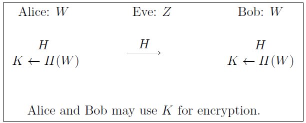
Figure 2: Privacy Amplification
However, this scheme is only secure against an eavesdropping only adversary. An active adversary may temper with the message sent between parties, and easily make the two parties have inconsistent results. Prof. Yu then mentioned that using message authentication code, parties can detect message tempering. And that is also is the third problem of the second lecture’s problem set.
One-Time Message Authentication Code
By adding message authentication code (MAC), the receiving party can effectively detect tempering during the transmission with high probability. The third problem of the problem set in the previous lecture proposes a MAC scheme when the two parties share a secret and only use it once (ergo one-time). The scheme works as follows:
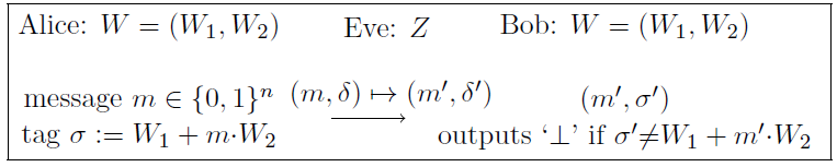
Figure 3: One-time MAC (IT-MAC)
The two parties of communication share a \(2n\) bit secret, denoted by \(W=(W_1,W_2)\), of which some information \(Z\) is leaked to an adversary. The average min-entropy of \(W\) conditioned on \(Z\) is at least \(n+t\), namely, \(\text{H}_\infty(W|Z) \ge n+t\). It can be proved that in this scheme, for any message \(m\), the adversary’s success probability
\[ \Pr_{(w_1,w_2)\gets W,z\gets Z}[m^\prime=A(m,\sigma,z):m\ne m^\prime\land\sigma^\prime=w_1+m^\prime\cdot w_2]\le 2^{-t}. \]
However, as Prof. Yu mentioned in his lecture, the min-entropy of the shared secret is at least \(n+t\) bits, while the constructed scheme can only guarantee at least \(t\) bit of security (I do not know for sure such notion is correct, but from the $ε$-secure notion in the previous lecture I am confident about that). In other words, there is a \(n\) bit entropy loss. He then stated by using pseudorandomness, such problem can be solved.
Modern Cryptography: Computational Approach
The content of the third handout starts from here, meaning the previous contents focus on perfect or statistical security, which although being secure against all-mighty adversaries, is utterly inefficient in practice. In particular, notice that the key space of a perfectly-secure encryption scheme has to be at least as large as its message space. This means that if we consider the key and message as binary strings, the key must be at least as long as the message, and that is obviously ineffective.
The modern approach of cryptography (i.e. the computational-complexity based approach) resolves this problem by relaxing the notion of security, in particular, only requiring security against efficient adversaries (since the asymptotic notion is considered in most cases, this means the advantage of the adversary ends in time polynomial in the security parameter). In this way, not only the efficiency can be improved, but also many other interesting and useful constructions can be built. (Recall that in the first course of Prof. Liu’s Modern Cryptographic Algorithm, it is explained that assuming one-way function exists, the entire symmetric cryptography can be constructed, e.g. pseudorandom generator, IND-CPA secure encryption etc.)
The lecture has different focus with the third handout. In particular, the handout proved several facts concerning the indistinguishability encryption test in the KL book, namely, any \(\mathsf{PPT}\) adversary cannot guess with probability better than negligible one bit of the plaintext given the ciphertext in an indistinguishable encryption scheme. Another fact is one very similar to semantic security, except that auxiliary information is not considered. Once again, the Prof. Yu proves in the handout that the indistinguishability definition implies this semantic security-like definition. But the proof of the equivalence between indistinguishability and semantic security was not mentioned in the handout. I think in the lecture all of the above content was gone through in less than five minutes. The focus here was on computational-indistinguishability (the more general definition, on any distributions) and pseudorandom generator (which comes with the first hybrid argument proof).
Computational Indistinguishable Encryptions
Similar to the definition in the previous lecture, we define the indistinguishability experiment for private-key encryption scheme \(\mathcal{P}i = (\mathsf{Gen},\mathsf{Enc},\mathsf{Dec})\) with respect to \(\mathsf{PPT}\) adversary \(A=(A_1,D)\) here.
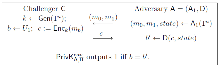
Figure 4: Symmetric Key Encryption Security Experiment
Note that in this experiment, since \(A\) is not all-mighty, and could use randomness in \(A_1\), state information (e.g. random coin used) is passed from \(A_1\) to \(D\). We call the encryption scheme \(\mathcal{P}i = (\mathsf{Gen},\mathsf{Enc},\mathsf{Dec})\) has indistinguishable encryptions in the presence of an eavesdropper if for all \(\mathsf{PPT}\) adversaries \(A\), there exists a negligible function \(negl(\cdot)\) such that \(\Pr[\mathsf{PrivK}_{A,\mathcal{P}i}^{eav}=1]\le 1/2 + negl(\kappa)\), the probability is over the choice of key \(k\), bit \(b\), randomness used in the encryption, and randomness used in \(A\). An alternative way of defining this is to state that for all \(\mathsf{PPT}\) adversaries \(A\), there exists a negligible function \(negl(\cdot)\) such that \(\Pr[D(1^\kappa,\mathsf{Enc}_k(m_0),state)=1]-\Pr[D(1^\kappa,\mathsf{Enc}_k(m_1),state)=1]\le negl(\kappa)\), where \((m_0,m_1,state)\gets A_1(1^\kappa)\). The proof is similar to the one in the previous lecture. One point to note though, is that in the previous proof, \(m_0\) and \(m_1\) are arbitrary so long as they are not identical. This is because the definition considered all possible adversaries, and therefore it is equivalent to the case when \((m_0,m_1)\gets A_1(1^\kappa)\).
Pseudorandom Generator
The definition of pseudorandom generator is as follows. Let \(l(\cdot)\) be a polynomial and let \(g\) be a deterministic polynomial-time algorithm such that upon any input \(s\in\{0,1\}^n\), the algorithm \(g\) outputs a string of length \(l(n)>n\). We say that \(g\) is a pseudorandom generator (PRG) if for all \(\mathsf{PPT}\) distinguishers \(D\), there exists a negligible function \(negl(\cdot)\) such that
\[ |\Pr[D(g(U_n)=1)-\Pr[D(U_{l(n)})=1]|\leq \mathsf{negl}(n), \]
where the probability is take over the random coins used by \(D\) and \(U_n\) (respectively \(U_{l(n)}\)). The difference between the output and input lengths \(l(n)-n\) is called the stretch factor of \(g\).
An Alternative Definition of PRG’s Security
Prof. Yu then introduced an alternative definition of PRG, namely \((t,\varepsilon)\) n-secure PRG. This is similar to the \((t,\varepsilon)\) -indistinguishable encryption in the handout. The definition states that if for any \(\mathsf{PPT}\) distinguisher \(D\) of running time at most \(t\), the advantage of the distinguisher on \(g(U_n)\) and \(U_{l(n)}\) is at most \(\varepsilon\). Prof. Yu then mentioned that when setting the parameters \(t=n^{\omega(1)}\) and \(\varepsilon=n^{o(1)}\), the two definitions are equivalent. (Right now I am convinced that \((t,\varepsilon)\) -secure implies the previous definition, but remain skeptical whether it is possible to construct an advantage that becomes non-negligible when \(t\) becomes super-polynomial. But this seems not worthy of pursuing compared to the definitions and hybrid argument to be introduced later.)
At this point, Prof. Yu mentioned in the lecture (and also in the handout), that PRG’s security is only guaranteed against efficient adversaries. Consider \(g:\{0,1\}^n\to\{0,1\}^{l(n)}\) as a PRG and an adversary \(D: x\mapsto x\in g(\{0,1\}^n)\), then the advantage of the adversary is
\begin{align*} \Pr[D(g(U_n))=1]-\Pr[D(U_{l(n)})=1] &= 1 - |g(\{0,1\}^n)|/2^{l(n)}\\ &\ge 1-2^{n-l(n)}\\ &\ge 1/2\enspace. \end{align*}
The last inequality holds since the stretch of the PRG is at least \(1\). This means the distinguisher \(D\) has constant advantage, and therefore the PRG \(g\) is definitely not secure in this case.
Replacement Lemma
The \((t,\varepsilon)\) -security of PRG enables a very versatile lemma called replacement lemma. I remember Prof. Yu mentioned this some afternoon in the lab the year before. He wrote this on the window of the lab and I remembered he asked someone to answer that. Anyway, the lemma states that if distribution \(X\) and \(Y\) is \((t,\varepsilon)\) -indistinguishable, and function \(f\) (defined over the union of the two distributions’ sample space) is \(T\) -computable, then the derived distribution \(f(X)\) and \(f(Y)\) is at least \((t-T,\varepsilon)\) -indistinguishable.
The proof is actually rather simple. Suppose that the result does not hold, then by contradiction, there exists a distinguisher \(D\) that runs in time at most \(t-T\), and distinguishes the two distributions with probability larger than \(\varepsilon\), namely \[ |\Pr[D(f(X))=1]-\Pr[D(f(Y))=1]|>\varepsilon. \] This already implies contradiction to the assumption. In order to see this, consider a distinguisher \(D^\prime(\cdot)=D(f(\cdot))\). This distinguisher will run in time at most \(t\), but will distinguish \(X\) and \(Y\) with probability greater than \(\varepsilon\). And therefore the distribution \(f(X)\) and \(f(Y)\) is at least \((t-T,\varepsilon)\) -indistinguishable.
Note that this lemma can be used to explain the replacement property of statistical distance. Prof. Yu explained this in brevity but I think I can elaborate a little here. First consider the equivalent definition of statistical distance as the maximum advantage among all distinguishers (no constraint on computational power here), and that could be roughly translated into \((\infty,\mathsf{SD}(X,Y))\) -indistinguishable. By applying substracting a \(T\) from the infinity limit of the running time, no actual limit is applied to the distinguisher. Now, we have when \(\mathsf{SD}(X,Y)\ge \varepsilon\), \(f(X)\) and \(f(Y)\) are at least \((\infty,\varepsilon)\) -indistinguishable, the advantage of any distinguishers on these two distributions is at most \(\varepsilon\). By the fact that the maximum of advantage is just statistical distance, we get \(\mathsf{SD}(f(X),f(Y)) \le\varepsilon=\mathsf{SD}(X,Y)\).
Stretching the Output Length of PRG: Hybrid Argument
By sequentially composing PRG to itself, a PRG with small stretch can be extended to get arbitrarily long pseudorandom bits. This is presented in the following lemma.
Let
\begin{align*} g:\{0,1\}^{n}&\to\{0,1\}^{n+s(n)}\\ s_i&\mapsto(s_{i+1},r_{i+1})\enspace, \end{align*}
where \(s_i,s_{i+1}\in\{0,1\}^n\), \(r_{i+1}\in\{0,1\}^{s(n)}\) be a \((t(n),\varepsilon(n))\) -secure PRG, and for any \(q(n)\in\mathbb{N}\), define
\begin{align*} g^q:\{0,1\}^n&\to\{0,1\}^{n+q(n)s(n)}\\ s_0&\mapsto(s_{q(n)},r_{q(n)},r_{q(n)-1},\ldots,r_1)\enspace, \end{align*}
where for \(0\le i\le q(n)-1\), iteratively compute \((s_{i+1},r_{i+1}):=g(s_i)\). Then, we have that \(g^{q(n)}\) is a \((t(n)-q(n)\cdot\mathsf{poly}(n), q(n)\cdot\varepsilon(n))\) -secure PRG, where \(\mathsf{poly}(n)\) is the running time of computing function \(g\).
The proof of this lemma demonstrated hybrid argument, which is extensively used in the field of cryptography. And since this is the first time it appears, it is worthwhile to pay more attention to that. I found that by using replacement lemma, some of the details of the proof in the handout can be hidden. The following is my slightly modified proof.
Like in the handout, we define the following distributions (note by placing the old output in the right hand side, the output of the function can be depicted as growing to the left, leaving pseudorandom stretches on the right hand side, and the notion actually aligned the seeds on the left hand side, the blank space on the right side can be filled with anything, so long as they are identically distributed, the adjacent two distributions will only have one iteration’s difference. I think this is the intuition behind constructing the series of distributions, a series of padded mimic snapshots along with the growth of the pseudorandom bits.)
\begin{align*} H_0&\overset{\text{def}}{=}g^q(U_n)\\ H_1&\overset{\text{def}}{=}(g^{q-1}(U_n),U_s)\\ H_2&\overset{\text{def}}{=}(g^{q-2}(U_n),U_{2s})\\ &\vdots\\ H_{q-1}&\overset{\text{def}}{=}(g(U_n),U_{(q-1)s})\\ H_{q}&\overset{\text{def}}{=}U_{n+qs}\enspace.\\ \end{align*}
After this, we can observe that for any \(i\in[q]\), the adjacent distributions \(H_i\) and \(H_{i-1}\) can be derived by applying $gq-i to the distribution in the assumption, namely, \(g(U_n)\) and \(U_{n+s}\), and padding \(U_{(i-1)s}\) to the right hand side of the random variables. By replacement lemma, \(g(U_n)\) and \(U_{n+s}\) is \((t,\varepsilon)\) -indistinguishable, then the resulting distribution is \((t-(q-i)\cdot\mathsf{poly}(n),\varepsilon)\) -indistinguishable, which implies it is \((t-q\cdot\mathsf{poly}(n),\varepsilon)\) -indistinguishable. Then by using the triangle inequality, we have for any probabilistic distinguisher \(D\) with running time no more than \(t-q\cdot\mathsf{poly}(n)\), the advantage of \(D\) distinguishing $H_0 and \(H_q\) is
\begin{align*} |\Pr[D(H_0)=1]-\Pr[D(H_q)=1]| &\leq \sum_{i=1}^q|\Pr[D(H_{i-1})=1]-\Pr[D(H_i)=1]|\\ &\leq q\cdot\varepsilon\enspace, \end{align*}
and that completes the proof.
18-19-2 Lecture 4
In this note, the content of this week’s lecture on provable security by Prof. Yu is summarized, from the handout and my own note taken at the lecture. This week’s lecture focuses on hardcore predicate of one-way function and Goldreich-Levin Theorem.
Lecture Content
In this lecture the main focus is on the theoretical construction of pseudorandom generators. Namely, a lemma concerning hardcore bit of one-way permutation implies pseudorandom generator (which works the other way as well) and Goldreich-Levin theorem were introduced. The proof of Goldreich-Levin theorem uses a concept called list decoding, which is a little mind-blowing for me. The lecture begins by giving hints on the last homework of the second lecture.
Equivalence Between Min-Entropy and Collision Entropy
In the first ten minute of the lecture, Prof. Yu explained to the class how to give answer to the fourth question of the homework in the second handout. The problem is that given a distribution \(X\) with collision-entropy \(\mathbf{H}_2(X)\geq k\), \(\forall\delta: 0< \delta <1\), it is possible to construct another distribution \(Y\) such that \(\mathbf{H}_\infty(Y)\geq k-\log(1/\delta)\), and \(\mathsf{SD}(X,Y)\le \delta\).
The answer to this question is given in the note of lecture 2. I think Prof. Yu’s answer implies that the rest of the set \(S:=\{x|\Pr[X=x]>1/\delta\cdot2^{-k}\}\) can be ignored in the distribution of \(Y\). However, I think this will make the question rather disappointing, since constructing another distribution over the exact sample space of \(X\) seems like a stronger guarantee. This is why I argued about the upper bound of minimum probability in the previous answer. This guarantees that when putting the extra probability to the probability over the set \(S\), there exists an assignment that does not exceed the maximum probability requirement \(\Pr[Y=x]\le 1/\delta\cdot2^{-k}\).
Another point to note is that the result \(\Pr[X\in S]<\delta\) can be treated as the result of Markov’s inequality. This is because we can treat the collision probability as the expectation of random variable \(\Pr[X]\), which is no more than \(2^{-k}\). And ergo the result.
One-Way Functions and Permutations
The definition of one-way function here is the same with that given in Prof. Liu’s lecture. Namely, given a function family \(f:\{0,1\}^{n}\to\{0,1\}^{l(n)}\) is a one-way function ensemble if it is
Easy-to-Compute: \(f\) can be computed by some algorithm in time \(\mathsf{poly}(n)\),
Hard-to-Invert: for every \(\mathsf{PPT} A\), there exists a negligible function \(negl(\cdot)\) such that
\[ \Pr_{X\gets U_n,x^\prime\gets A(1^n,f(X))}[f(x)=f(x^\prime)]\le negl(n). \]
Despite the similarity, Prof. Yu did argued in the handout that the more formal definition, where the domain and ranges are arbitrary sets and explicit sampling algorithms may be needed to sample a random element over the domain.
An Intuitive Interpretation of Implication
The relationship between one-way function exists (denoted by \(\mathsf{OWF}\)) and \(\mathcal{P}\ne\mathcal{NP}\) was also mentioned in the class. \(\mathsf{OWF}\) implies \(\mathcal{P}\ne\mathcal{NP}\), or written in a more standard form, \(\mathsf{OWF}\le\mathcal{P}\ne\mathcal{NP}\). In my intuitive opinion, this can be interpreted as there are two big truth tables with some entries’ value unknown. But from some evidence we can conjecture that they are true. Now the stronger assumption (the one that implies others) has more entries that are conjectured correct, and the ones that need to be conjectured correct is only a subset of the first one. This already explained the first one’s conjecture correctness implies the second one’s correctness. What’s more, if by contradiction, an entry of the second one is wrong (contradicting the assumption), then we can surely say that the first conjecture is not correct (since all the conjectured entries need to be correct to make the assumption correct), which also means that the contradicting entry is more ’lethal’ than the other entries outside the subset in the first assumption. Since finding a more powerful false entry is harder, this explains why intuitively, the implies sign ‘\(\le\)’ can be understood as “the hardness is lesser or equal than”.
One-Way Functions based on Different Assuptions
There are different assumption on which one-way functions can be constructed. Some of them are listed in the handout, they are
- Integer Factorization,
- Subset Sum, and
- Discrete Logarithm.
The first and third one have been extensively studied and tested in practice.
Hard-core Predicates of One-Way Functions
The definition of hard-core predicate is as follows. A polynomial-time computable predicate \(h_c:\{0,1\}^n\to \{0,1\}\) is called a hard-core predicate of a function \(f\) if for every \(\mathsf{PPT}\) algorithm \(A\), there exists a negligible function \(negl(\cdot)\) such that \[ \Pr_{X\gets U_n}[A(1^n,f(X)=h_c(X)]\leq 1/2+negl(n), \] where the probability is take over the choice of \(X\) and the random coins of \(A\).
Note that hard-core predicate exists implies one-wayness. The following theorem states that for one-way permutations, hard-core predicates imply the explicit construction of pseudorandom generators. The theorem is as follows.
If a permutation \(f:\{0,1\}^n\to\{0,1\}^n\) has a hard-core predicate \(h_c:\{0,1\}^n\to\{0,1\}\), then the function \(g(x) = (f(x),h_c(x))\) is a pseudorandom generator with a single bit stretch.
The proof given in the handout concerns deterministic distinguisher of pseudorandomness, and imposes stronger limit to the distinguisher of pseudorandomness (in that proof if the hard-core predicate is \((t(n),\varepsilon(n))\) -hard then the output of \(g(\cdot)\) is \((t(n)/2,\varepsilon(n))\) -indistinguishable from \(U_{n+1}\)). I tried to improve the proof by concerning \(\mathsf{PPT}\) adversaries and remove the loss in running time limit. The proof is as follows.
Suppose by contradiction, there is a \(\mathsf{PPT}\) adversary \(A\) of running time \(t(n)\) that can distinguish pseudorandomness such that
\[ \Pr_{X\gets U_n}[A(f(X),h_c(X))=1]- \Pr_{X_1\gets U_{n}, X_2\gets U_1}[A(X_1,X_2)=1]> \varepsilon(n)\enspace. \]
Observe the latter probability can be written as \[ 1/2\cdot\Pr[A(X_1,h_c(X_1))] + 1/2\cdot\Pr[A(X_1,1\oplus h_c(X_1))], \] which means \[ 1/2\cdot\Pr_{X\gets U_n}[A(f(X),h_c(X))=1]-1/2\cdot\Pr[A(X_1,1\oplus h_c(X_1))]>\varepsilon(n)\enspace. \] Now construct a \(\mathsf{PPT}\) algorithm \(D\) that computes the hardcode bit of input, given the output of the one-way permutation. After \(D\) gets its input \(f(X)\), it samples a random bit \(b\gets U_1\), and then calls \(A\), and get \(b^\prime \gets A(f(X),b)\). If \(b^\prime = 1\), output \(b\); else, output \(1\oplus b\).
The probability that \(D\) succeed is as follows,
\begin{align*} \Pr_{X,b,r}[\text{D wins}]&=\Pr[b=h_c(X)]\cdot \Pr[b^\prime=1|b=h_c(X)]+\Pr[b=1\oplus h_c(X)]\cdot \Pr[b^\prime=0|b=1\oplus h_c(X)]\\ &=1/2\cdot\Pr[A(f(X),h_c(X))=1]+ 1/2\cdot(1-\Pr[A(f(X),1\oplus h_c(X))=1])\\ &>1/2 + \varepsilon(n)\enspace. \end{align*}
And that contradicts the assumption that \(h_c(\cdot)\) is a (\(t(n)\),\(\varepsilon(n)\))-hard-core predicate for one-way permutation \(f\).
Reverse Thinking
Note that the previous theorem essentially states that next bit unpredictability implies pseudorandomness. Actually the result works in the other direction as well. Namely, for a pseudorandom generator \(g:\{0,1\}^n\to\{0,1\}^{l(n)}\), \(\forall i \in [l(n)-1]\), \(\forall \mathsf{PPT} A\), there exists a negligible function \(negl(\cdot)\), such that \[ \Pr_{X\gets U_n}[A(f(X)_{[1:i]})=f(X)_{[i+1]}] \le 1/2 + negl(n). \] This is actually quite trivial (which I failed to realize after it was brought up in class, when Prof. Yu noticed me mumbling, as if I knew how to prove it, but it turned out I could not present the complete answer). Suppose that there exists some position \(i\) and a algorithm $A that satisfies the above probability’s negation, then for the construction of pseudorandom distinguisher \(D\), apply the first \(i\) bits of the input to \(A\) and output \(1\) if the predicted bit equals \(f(X)_{[i+1]}\). The probability of \(D\) outputting \(1\) in the case of real randomness is \(1/2\), and in the pseudorandom case, it is \(\Pr_{X\gets U_n}[A(f(X)_{[1:i]})=f(X)_{[i+1]}]\). It is obvious that the advantage of the adversary is non-negligible.
Universal Construction of Hard-Core Predicates: Goldreich-Levin
Theorem
Digested from the handout, we have “It was conjectured that every one-way function has a hard-core predicate, and this was proven by Goldreich and Levin in STOC 1989.” Prof. Yu mentioned that the creativity of this proof is that it uses Chebyshev’s inequality instead of Chernoff bound, which does not require all components are independent, but only pairwise independent. And that reduces the number of guesses needed in the proof, and therefore increases the success probability as well.
The proof given in the handout is the complete proof, unlike in the KL book, where the proof is given in steps, first a simplified case, then the full proof. Prof. Yu did managed to organize the proof in separate independent modules. There are mainly two techniques in this proof, in my opinion. The first one is how to use list decoding to convert a couple of guesses of the hard-core bit into an inversion of the preimage with high probability (\(1/2\) to be specific). The other one is to use Chebyshev’s inequality instead of Chernoff bound, which could reduce the number of guesses needed, ergo increasing the success probability of the inversion algorithm.
There is one remaining problem to be solved. I think the number of guesses \(l=\lceil\log(1+2n/\varepsilon(n)^2)\rceil\) does not guarantees \(2^{-l}\ge\varepsilon(n)^2/4n\) (although $2-l≥ε(n)^2/8n can be guaranteed).
The proof is as follows. Suppose by contradiction there exists a \(\mathsf{PPT}\) algorithm \(A\) such that \[ \Pr_{x\gets U_n,r\gets U_n}[A(f(x),r)=\mathsf{gl}(x,r)]>1/2+\varepsilon(n), \] where the probability is taken over the choice of \(x, r\) and the internal random coins of \(A\). We first argue there exists a set \(S\) of size \(|S| \ge \varepsilon(n)/2\) such that \(\forall x \in S, \Pr_{r\gets U_n}[A(f(x),r)=\mathsf{gl}(x,r)]>1/2+\varepsilon(n)/2\). This is due to Markov’s inequality (not the normal form, since the direction of inequality is inversed). Note that
\begin{align*} \Pr_{x\gets U_n,r\gets U_n}[A(f(x),r)=\mathsf{gl}(x,r)] &=\sum_{x}\Pr[X=x]\cdot\Pr_{r\gets U_n}[A(f(x),r)=\mathsf{gl}(x,r)]\\ &\le\Pr[X\not\in S]\cdot(1/2+\varepsilon(n)/2)+\Pr[X\in S]\\ &\le 1/2+\varepsilon(n)/2 +\Pr[X\in S]\enspace, \end{align*}
which means \(\Pr[X\in S]\ge \varepsilon(n)/2\). Conditioned on \(X\in S\), we construct the following efficient algorithm that can invert \(f\) given \(f(x):x\in S\) with probability no less than \(\varepsilon(n)^2/16n\) (in the handout this is \(\varepsilon(n)^2/8n\) but I think that might have a tiny problem). This reduces our problem to constructing such an algorithm.
The inversion algorithm \(A^\prime\) works as follows. (Let \(l = \lceil\log(2n/\varepsilon(n)^2+1)\rceil\).)
- Uniformly and independently samples \(s^1,\ldots,s^l\gets U_n\), and \(\sigma^1,\ldots,\sigma^l\gets U_1\), where \(\sigma^i\) is a guess for \(\mathsf{gl}(x,s^i)\).
- For every non-empty subset \(\mathcal{I}\subseteq [l]\), let \(r^{\mathcal{I}}\overset{\text{def}}{=}\mathop{\oplus}_{i\in\mathcal{I}}s^i\), \(\tau^{\mathcal{I}}\overset{\text{def}}{=}\mathop{\oplus}_{i\in\mathcal{I}}\sigma^i\). Each \(\tau^{\mathcal{I}}\) is a guess for \(r^{\mathcal{I}}\), because if all the \(\sigma^i\)’s are correct guesses, the resulting \(\tau^{\mathcal{I}}\)’s are also correct guesses.
- For every \(j \in [n]\), make a guess about the \(j^{\text{th}}\) bit
of input \(x\), denoted by \(x_j\), as follows:
For every non-empty subset \(\mathcal{I}\subseteq [l]\), set \(v_j^{\mathcal{I}}:=\tau^\mathcal{I}\oplus A(f(x),r^{\mathcal{I}}\oplus e_j)\), where
\[ e_j \overset{\text{def}}{=}\underbrace{0\ldots0}_{j-1} 1\underbrace{0\ldots0}_{n-j}. \]
Do a majority voting on candidate values \(\{v_j^{\mathcal{I}}:\emptyset \ne\mathcal{I}\subseteq[l]\}\), and let \(x_j^\prime\) be the majority bit of them.
Now we claim that conditioned on \(x \in S\), the success probability of \(A^\prime\) is over \(\varepsilon(n)^2/16n\). First of all, The probability of \(\sigma^1,\ldots,\sigma^{l}\) all being correct guesses is $2-l which is greater than \(\epsilon(n)^2/8n\) (this is where the divergence comes from). Conditioned on that, we now analyze the probability that voting on bit \(x_j\) succeeds. Recall that we have already proved
\begin{align*} \Pr_{X\gets U_n}[A^\prime(f(X)) = X]&\ge\Pr_{X\gets U_n}[X\in S]\cdot\min_{x\in S}\Pr[A^\prime(x)=x]\\ &\ge \varepsilon(n)/2 \cdot\varepsilon(n)^2/8n \cdot\min_{x\in S} \Pr[x^\prime_1=x_1\land x^\prime_2=x_2\land\ldots\land x^\prime_n=x_n]\\ &=\varepsilon(n)/2 \cdot\varepsilon(n)^2/8n\cdot (1- \min_{x\in S} \Pr[x^\prime_1\ne x_1\lor x^\prime_2\ne x_2 \lor\ldots\lor x^\prime_n\ne x_n])\\ &\ge\varepsilon(n)/2 \cdot\varepsilon(n)^2/8n\cdot (1- \sum_{i\in[n]}\Pr[x^\prime_i\ne x_i])\enspace, \end{align*}
where from the second line the probability is conditioned on all \(\sigma^i\)’s are correct guesses and the last inequality is from union bound and the requirement of \(x\) is from the previous equation. It suffices to prove for any \(x\in S\), \(\Pr[x^\prime_i\ne x_i]\le 1/2n\) for all \(i\in [n]\), and we will prove it below.
Note that in the third step of \(A^\prime\), if the \(j^{\text{th}}\) bit of \(x\) is \(0\), then adding \(e_j\) to \(r^{\mathcal{I}}\) does not change the hard-core bit, and the output \(v_j^{\mathcal{I}}\) will be \(0\). On the other hand, if \(x_j = 1\), then the output will be inverted and \(v_j^{\mathcal{I}}=1\). This means \[ \Pr[v_j^{\mathcal{I}}\text{ is correct}] = \Pr[A(f(x),r^{\mathcal{I}}) = \mathsf{gl}(x,r^\mathcal{I})] \ge1/2+\varepsilon(n)/2. \] Let \(m = 2^{l}-1 > 2n/\varepsilon(n)^2\), which is the number of candidates for the majority voting, and denote \(\mathsf{E}^\mathcal{I}\) be the event that \(v_j^{\mathcal{I}}\) is correct. By the construction of \(r^{\mathcal{I}}\)’s, we have that they are pairwise independent. Now we analyze the probability of the event that less than half of the \(v_j^{\mathcal{I}}\)’s are correct, which is
\begin{align*} \Pr[\sum_{\mathcal{I}\in[l]}\mathsf{E}^{\mathcal{I}}<m/2] &= \Pr[\sum_{\mathcal{I}\in[l]}\mathsf{E}^{\mathcal{I}}-m\mu<m/2-m\mu]\\ &\le\Pr[\sum_{\mathcal{I}\in[l]}\mathsf{E}^{\mathcal{I}}-m\mu<-m\cdot\varepsilon(n)/2]\\ &\le\Pr[|\sum_{\mathcal{I}\in[l]}\mathsf{E}^{\mathcal{I}}-m\mu|>m\cdot\varepsilon(n)/2]\\ &\le \frac{Var(\sum_{\mathcal{I}\in[l]}\mathsf{E}^{\mathcal{I}})} {(m\cdot\varepsilon(n)/2)^2}. \end{align*}
The last inequality is due to Chebyshev’s inequality. Note that since each two \(\mathsf{E}^{\mathcal{I}}\)’s are pairwise independent, this means
\[ Var(\sum_{\mathcal{I}\in[l]}\mathsf{E}^{\mathcal{I}}) = \sum_{\mathcal{I}\in[l]}Var(\mathsf{E}^{\mathcal{I}}) \le m\cdot 1/4. \]
Bringing that to the equation above, we have
\begin{align*} \Pr[\sum_{\mathcal{I}\in[l]}\mathsf{E}^{\mathcal{I}}<m/2] &\le \frac{Var(\sum_{\mathcal{I}\in[l]}\mathsf{E}^{\mathcal{I}})}{(m\cdot\varepsilon(n)/2)^2}\\ &\le\frac{m\cdot1/4}{m^2\cdot\varepsilon(n)^2\cdot1/4}\\ &\le\frac{1}{2n/\varepsilon(n)^2\cdot\varepsilon(n)^2}\\ &=1/2n. \end{align*}
And that completes the proof of Goldreich-Levin Theorem.
A Central Theorem in Cryptography
The previous two lemma combined gives us the result one-way permutation implies pseudorandom generators. In fact, a more general statement that one-way function implies pseudorandom generators is also true. This is proved by Håstad et al. in [HILL99]. The proof is much more involved and not suitable for this lecture. Prof. Yu mentioned in class that this construction is more of theoretical interest than of practical value, since the loss in efficiency, although polynomial, is still very large. The simplified cases are that of one-way permutations (which has already been proved), and regular one-way functions (every image has the same number of preimages).
Homework
The handout of this lecture has five homework problems. The first one is to improve the advantage loss in the original proof. The rest of the problems are from KL book.
Improving the Advantage Loss in the Proof of Goldreich-Levin Theorem
What the previous proof proves is essentially assuming some algorithm \(A\) of running time \(t(n)\) can guess the hard-core bit with probability better than \(1/2 + \varepsilon(n)\), then there is another algorithm \(A^\prime\) of running time \(\mathsf{poly}(1/\varepsilon(n),n)\) that can compute \(x\) from \(f(x)\) with probability better than \(\varepsilon(n)^3/16n\) (which is non-negligible if \(\varepsilon(n)\) is). This is a stronger guarantee than the one required in one-wayness experiment, where only \(x^\prime \in f^{-1}(f(x))\) is needed. If we add a simple check after \(A^\prime\) output \(x^\prime\), and re-guess \(x\) with fresh randomness if \(f(x^\prime)\ne f(x)\), we can increase the success probability to \(\varepsilon(n)/4\).
There is a detail that need to be paid attention to in the previous argument. The first probability that \(x\in S\) only considers the very preimage \(x\), while in the modified proof, we need to consider all other preimages. Actually, this is not a problem, since the only information that \(A\) learns is \(f(x)\), and that is the same for all other preimages \(x^\prime \in f^{-1}(f(x))\). Conditioned on \(x\in S\), we can safely conclude that all other preimages are in \(S\).
The other point I think may be a caveat is that by repeating the guessing process, we need to calculate the expected running time of \(A^\prime\), since it’s halting is probabilistic now. This should not be a big problem, since the success probability of one guessing is more one over some polynomial, and the inverse is smaller than that polynomial, on infinitely many \(n\)’s. Despite this, the specific halting strategy should be specified to make sure \(A^\prime\) runs in polynomial time.
Exercise 6.1 from KL Book
For \(f(x,y) = x+y\), output \((x+y,0)\) on the output; for \(f(x)=x^2\), just use interpolation to find \(x\).
Exercise 6.2 from KL Book
Assuming \(f:\{0,1\}^n\to\{0,1\}^{l(n)}\) is a one-way function (family), it follows from one-wayness that for all \(\mathsf{PPT}\) algorithm \(A\), there exists a negligible function \(negl(\cdot)\) such that \[ \Pr_{X\gets U_n,x^\prime\gets A(f(X))}[f(x^\prime)=f(X)] < negl(n). \] Now construct another function \(f^\prime:\{0,1\}^n\to\{0,1\}^{l(n)}\) that behaves exactly like \(f\) except on \(x=0^n\), where it outputs \(0^{l(n)}\). For any \(\mathsf{PPT}\) algorithm \(A\), the success probability of inverting \(f^\prime\) is
\begin{align*} \Pr_{X\gets U_n,x^\prime\gets A(f^\prime(X))}[f^\prime(x^\prime)=f^\prime(X)]\leq2^{-n}+\Pr_{X\gets U_n,x^\prime\gets A(f(X))}[f(x^\prime)=f(X)]\enspace, \end{align*}
which is still negligible. This means \(f^\prime\) is also a one-way function. The KL book maybe tries to tell me one-wayness is a statistical result, changing one term will not essentially change the overall characteristics.
Exercise 6.4 from KL Book
The proof is trivial.
Exercise 6.6 from KL Book
If \(f(\cdot)\) is a one-way function, then \(g(x) = f(f(x))\) is a one-way function. This is because \(f\) is efficiently computable, and therefore it is easy to construct an algorithm to invert \(f\) given an algorithm to invert \(g\). The second part is essentially the same.
Pilot Course
Basic Information
- Lecturers: 郁昱, 刘振
- Canvas website: oc.sjtu.edu.cn/courses/19984
Outline
Testing Signing in (not accounted as score reference)
- Since this is only a testing course, absence will not be penatied.
Testing Zoom website
Begin at exactly 8:55
15 students enrolled
Class Outline
- Classical Cryptography
- Modern Cryptography
- Post-quantum Cryptography
- Concluding Remarks
Natural Proof: inbetween area between security and insecurity.
Correspondence between crypto, complexity and math
| Cryptography | Complexity | Math |
|---|---|---|
| PRG, Stream Cipher | PRG, Derandomization | |
| PRF, Block Ciphers, Authentication | Hardness of learning, Natural proof barrriers | |
| Privacy amplification | Randomness extraction | Expanders, Ramsey Graphs |
| Succinct ZK arguments | PCP, Locally testable Codes | |
| Leakage-resilient crypto | Dense model theorems, hardcore sets | primes in arithmetic progression |
| Obfuscation | Hard search problems | |
| private information retrieval | locally decodable codes | extremal set theory |
| HE, homomorphic secret sharing | locally random reductions, program checking |
Lecture 1
Introduction
Not all slides will be uploaded to canvas prior to the lecture.
Provable security is an important aspect of modern cryptography.
Prerequisites:
- read formal proofs
- analyze complexity of algorithms
- familiarity with basic probability theory
Textbooks:
- KL book
- Foundations of cryptography
- research papers
What is Cryptography
Cryptography is a part of modern theoretical computer science. Pseudorandomness, communication complexity, and ZK are also useful tools in TCS in general.
Godel prize topics:
- Natural proof – problems that are hard to prove or disprove, natural proof proves that the proof itself is hard.
Cryptography is not all like mathematics. In crypto, people are only concerned with moderate problems, and efficient algorithms.
More on that table:
| Cryptography | Complexity | Math |
|---|---|---|
| PRG, Stream Cipher | PRG, Derandomization | |
| PRF, Block Ciphers, Authentication | Hardness of learning, Natural proof barrriers | |
| Privacy amplification | Randomness extraction | Expanders, Ramsey Graphs |
| Succinct ZK arguments | PCP, Locally testable Codes | |
| Leakage-resilient crypto | Dense model theorems, hardcore sets | primes in arithmetic progression |
| Obfuscation | Hard search problems | |
| private information retrieval | locally decodable codes | extremal set theory |
| HE, homomorphic secret sharing | locally random reductions, program checking |
Classic Cryptography
Traditionally the definition is about secure communication, while the modern verison is more versatile.
Basic primitives:
- one-way function: for randomly chosen pre-image, it is hard to find any pre-image correponding to the image.
- pseudorandom generator: randomness amplification
- pseudorandom function: PRG, but even better
Some basic tasks:
- encryption: transformation of message that protects message against evasdroppers
- MAC/Signature: protect message integrity the previous is the symmetric case while the latter one is public-key case
- Secure computation: protect input privacy while preserving functionality
Applications:
- Secure communication
- authetication
- digital signature (MAC, but better)
- privacy-preserving computation: MPC, HE, Obfuscation, etc.
Obfuscation originates from software code protection, crypto community wants to formalize it and enhance upon it, but so far no satisfying results.
- Combination of previous tools
Symmetric Key Encryption (SKE)
A triplet of algorithms
- Key Generation: \(k \gets KeyGen(1^\kappa)\)
- Encryption: \(c \gets Enc(m, k)\)
- Decryption: \(m^\prime \gets Dec(c, k)\)
Symmetric in the sense that the two parties share common secret knowledge beforehand.
Properties:
- Correctness: BPP or P
- Security: passive or active, computaitonally bounded or unbounded (not like oracles)
Examples in classical cryptography:
Caesar Cipher, Enigma
Shannon’s OTP
Just operations on the GF2 field. Perfectly secure in the sense that ciphertext is independent of message. In other words, the mutual information between ct and message is zero.
Perfect secrecy’s limitation: \(|K| = |M|\)
Shannon’s Entropy
\(H = \sum_i p_i \cdot \log(1/p_i)\) \(I(X;Y) = H(X) - H(X|Y)\)
Adversarial Model
- Cihpertext-only attack
- known-plaintext attack
- chosen-plaintext attack
- chosen-ciphertext attack
How to argue security
Using reduction based proofs. If problem A is computationally hard, then crytpo system B is secure against PPT adversaries. In practice, this is done through showing that algorithm for B can be efficiently converted to algorithm for A.
Public Key Cryptogrpahy
Also a triplet of algorithms
- Keygen
- Encryption
- Decryption
Definition of security: CPA game.
Modern Cryptography
Modern crypto bases security upon computationally hard problems, which is what PKE do. But SKE normally does not have this requirement (e.g. AES, DES).
The dawn of modern cryptogrphy: DH, RSA.
Decisional DH assumption: \((g^x, g^y, g^{xy}) \sim (g^x, g^y, g^z)\)
Pseudorandomness to break shannon’s barrier: BMY generator (hybrid argument)
The hierarchy of cryptography
- Algorithmica: \(\mathcal{P}=\mathcal{NP}\)
- Heuristica: \(\mathcal{P}\neq \mathcal{NP}\)
- Pessiland: no OWF
- Minicrypt: exists OWF
- Cryptomania: exists PKC and MPC
One-way functions: the minimal assumption for cryptography. Notice this is in the average case sense. HILL theorem states that OWF implies PRG.
Not all cryptographic primitive has secret
CRHF: hard to find collision for a random instance of hash function. \[\Pr_{h\gets H}[A(h)=(x,x^\prime): x\neq x^\prime, h(x) = h(x^\prime)]\]
Practical instantiations of CRHF: MD5, SHA1, SHA256, SHA3
But what about a family of algorithms? This is due to definitional problems.
Two party computation
Garbled circuit in [Yao82b]. For practical application, c.f. Netherland sugar beat auction case.
The Quantum CRYSIS
- Shor’s algorithm: solves DL and Factoring in poly-time
- Grover’s algorithm: general quadratic speed-up
It is believed that \(BQP \ne NP\).
NIST PQC candidate announcement.
``GOOD’’ assumptions include:
- Lattice-based: e.g. LWE
- Code-based: e.g. LPN
- Hash-based: limited to digital sinature
- Multivariate: no provable security?
LWE and LPN problem, solving noisy equations over finite-field, similar to solving equations over finite-field (plain elimination) or solving noisy equations over infinite-field (projection), but actually different.
Decoding Random Linear q-ary codes. Message is \(s\), generation matrix is \(A\), noisy codeword is \(A \cdot s + e\). This problem is NPC in the worst case, also hard in the average case (the famous reduction).
LPN: sub-exponential algorithm exists but that’s all for the status quo. BKW: time complexity is \(2^{n/\log n}\) for constant noise rate.
LPN-based PKE (one-bit)
Alice (the receiver): \(a\gets \{0,1\}^{n\times n}\), \(sk = s^T\), \(e^T \gets B_\mu^n\) \(pk = (a, s^T \cdot a + e^T)\)
Bob (the sender): \(s_1,e_1\gets B_\mu^n\) \(c_1 = a\cdot s_1 + e_1\), \(c_2 = b^T \cdot s_1 + m\)
Security is easy to prove since all the messages are LPN instances or hard core bits.
Piling-up lemma: for \(x,y\gets B_\mu^{2n}\): \(\Pr[x^T\cdot y = 0]\ge 1/2 + 2^{O(-n\mu^2)}\).
Lecture 2
Recaping Last Lecture
CRHF
Hard to find collision, and it can be based on several mathematical assumptions. Another caveat is that in this definition, we consider a family of functions \(\mathcal{H}\), while in practice we only have only one algorithm, e.g. SHA256, MD5.
Note that in non-uniform model the collision can be modelled as auxiliary input, and thus the one-algorithm definition can be trivially broken.
Multiparty Computation
Nothing is leaked beyond the input and output information.
Decoding Random Linear Code
Lattice / LPN based assumptions are these types of assumption. The latest achievement based on these assumptions are Gentry in STOC 2009.
Introducing the homomorphic evaluation function \(\mathsf{Eval}(pk, f, c_1,\ldots,c_t)\)
Important Limitation: Complexity of decrypting \(c^*\) must not depend on the complexity of \(f\). Otherwise, one trivial solution is to keep all the ciphertext inputs and the description of function f, then in decryption, just decrypt and then evaluate. This goes against the goal of computation outsourcing.
Cryptography is full of conjecture, surprisingly equivalence, and impossibility results.
A good / famous example is Alice’s Jewelry Store. Worker (server) works (evaluates) on raw materials (inputs) to produce jewelry (output).
This is like MPC, but only one round of communication, very efficient in communication.
Pre-2009 schemes are so called somewhat homomorphic, not fully.
Preliminaries of Provable Security
Writing a formal proof
- Conditionally
- by a reduction
- Unconditionally
- constructively or existentially
Most crypto proofs are conditional, the minimal assumption is the existence of one-way function. And the existence of OWF considers average-case hardness (most instances are hard), while \(\mathcal{P} \ne \mathcal{NP}\) considers worst case hardness.
Though seemingly groundless, conjectures like RSA seems robust enough. A French team successfully conducts cryptanalysis on ~ 800bits RSA.
Unconditionally proof usually involves information theory. Constructive results are surely more satisfying than existential solution (which only provides one-bit).
- Disproof
- provide one counterexample is sufficient
- Proof hard to prove
- shows that the proof itself is hard to come up with.
Examples
- Shows the number of primes are infinite Use simple proof technique
- For sequentially ordered primes \(p_1,\ldots,p_n\), is \(p_1\cdot p_2 \cdot \ldots \cdot p_n \pm 1\) prime as well? No, the prime list is not complete. Related problems are twin prime conjecture.
- Binary linear code. A binary (m,n)-code has dimension n and length m. The generator matrix is of size n by m.
Nearest Codeword Problem (NCP): given the generator matrix C and noisy codeword \(t^T = s^T \cdot C + x^T\). Noise x is limited by its hamming weight which is exactly \(d\). The solution is \(s^\prime\) such that
\[ s^T \cdot C + x^T = s^{\prime T} \cdot C + x^{\prime T} \]
Show most linear codes have unique decoding when codeword length \(m\) is large enough.
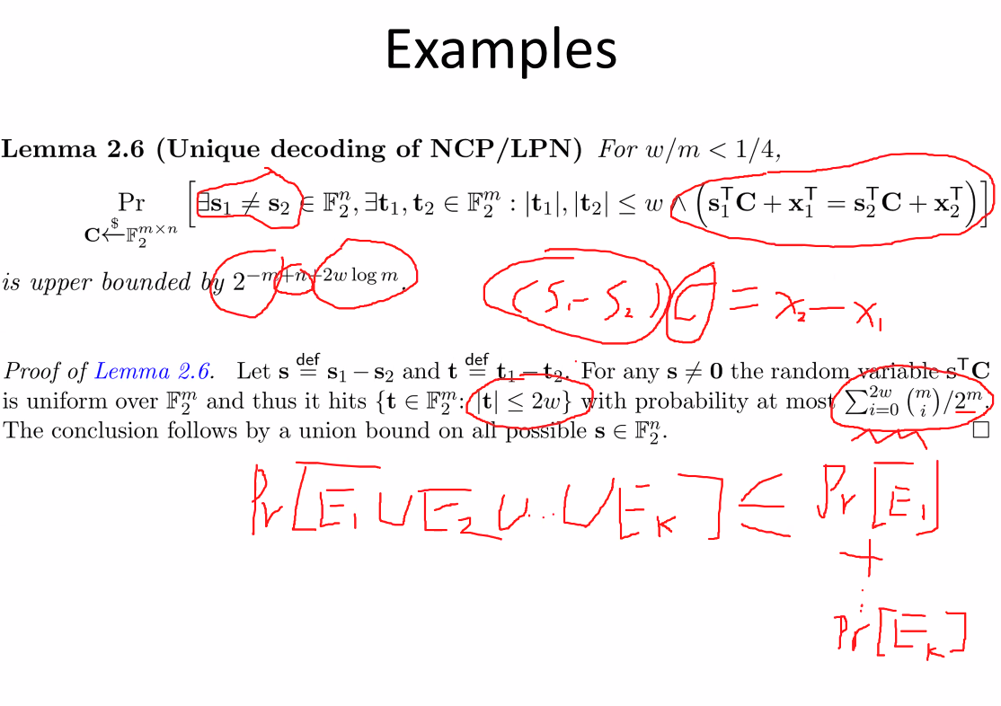
Figure 5: Proof of Unique Decoding of LPN
This is an example of existential probablistic proof.
Notations on rv’s and sets
Sets \(\{0,1\}\) is the most common one.
Notations of probability distribution
- non-negativity
- maps from sample space to real number in [0,1]
- add up to one
Random variables
very similar to distribution
Events and Independence
Event is actually a subset of sample space, independent events are two “regular” subspace. By regular I mean conditioning on one event the other one has the same probability.
Independent variables: for every possible value, the corresponding events are independent.
Polynomial and friends
Efficient algorithm means polynomial-time computable. In cryptogrpahy, we want the problem for adversary is super-polynomial hard while the success probability is some inverse of super-polynomial function.
A function \(f\) is superpolynomial if for every constant \(c>0\) and all sufficiently large \(n\) we have \(f(n) > n^c\).
Negligible function is the inverse of some superpolynomial. E.g. \(2^{n/2}\), \(n^{\log n}\)
Overwhelming and non-negligible
- overwhelming
- 1 - negligible
- non-negligible
- not negligible (larger than some polynomial for infinitely-many n’s)
- noticible
- larger than some inverse of polynomial
Example of non-negligible but non-noticible function: “punch-out” function at all even / odd points.
Asymptotic functions
big-oh notations.
| Asymptotic | Meaning |
|---|---|
| \(o\) | \(\leq\) |
| \(\omega\) | \(\geq\) |
| \(\theta\) | \(=\) |
| \(o\) | \(<\) |
| \(\omega\) | \(>\) |
Function Ensembles
Different functions for different problem scale.
Example: one-way function
Usual mathematical objects are functions of the security parameter.
Union bound and Markov inequality
Union Bound:
Markov Bound: \(\Pr[X \ge \delta \mathbb{E}[X] ]\le 1/\delta\)
Chebyshev’s Inequality
\[ \Pr[|X-\mu|\ge \delta\sigma] \le 1/{\delta^2} \]
Chernoff bound and Hoeffding Bound
There are additive form and multiplicative form
Piling up Lemma and misc
We have \(\Pr[\bar{x} = 1] = 1/2 - 1/2 \cdot (1 - 2\mu)^n\)
Extreme cases: \(\mu = 0\) nothing changes; one \(\mu = 1/2\) then the result is random.
- Fact 1.
- For any \(0\le x \le 1\) it holds that \(\log_2 (1+x) \ge x\). For any \(x > -1\) we have \(\log (1+x) \le x / \ln 2\)
- Fact 2.
- Binominal approximation
ANOTHER HOMEWORK on the existence of independent code
Lecture 3
How to do last lecture’s homework
If C is a random matrix, then Cr is uniformly random. The answer will not be distributed today, though.
Statistical distance / indistinguishability and the LHL
First define the indistinguishability experiment.
There are three levels of security:
- Unconditionally secure / information-theoretically secure
- advantage has zero advantage
- Statistically secure
- adversary has negligible advantage
- Computationally secure
- pseudorandomness, etc.
The experiment here is about private key encryption
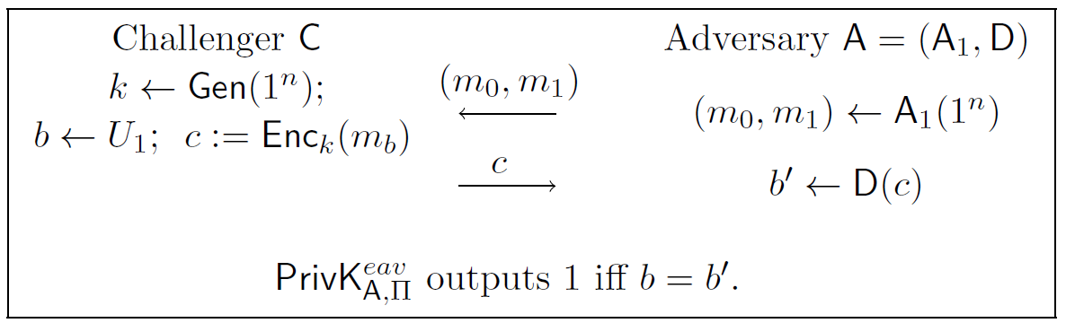
Figure 6: Private Key Encryption Experiment
The adversary’s advantage is \(\mathsf{Adv}{eav}{\mathcal{A},\mathcal{P}i} = \Pr[b^\prime = b] -1/2\) Notice here the adversary is considered to be all-powerful, and so it can determine which random coin is the most advantageous, and so it doesnot has to be a randomized algorithm, or to keep state information.
The above algorithm can also be transformed into an indistinguishability game, such that the same \(\varepsilon\) is still the bound. We can use conditional probability to prove this equivalence.
One-time pad is perfectly secure
OTP is defined over \(\{0,1\}^n\), we want to prove that this is perfect-secure. And it is so simple, since any two ciphertexts are distributed identically, so any adversary’s advantage is zero.
Statistical Distance
For two distributions X,Y, the statistical distance is defined as:
\[\mathsf{SD}(X,Y):=1/2 \sum_x \left|\Pr[X=x]-\Pr[Y=x]\right|\]
And we can define conditional statistical distance \(\mathsf{SD}(X,Y|Z):= \mathsf{SD}((X,Z),(Y,Z))\).
The 1/2 in the definition is to normalize the output to the range of [0,1].
SD provides a upper bound of the advantage of distinguishing two distributions. This can be seen as \(D\) defines a distribution on the support. The best we can do is to let it maximize the success probability (in the distinguishing game) on every input.
SD is a metric since it has:
- non-negativity
- identity of indiscernibles
- symmetry
- \(\mathsf{SD}(X,Z) \leq \mathsf{SD}(X,Y) + \mathsf{SD}(Y,Z)\) Furthermore, it has the following property:
- the equality holds when supports of \(X,Y\) are disjoint.
- for every function \(f\), \(\mathsf{SD}(f(X),f(Y))\leq\mathsf{SD}(X,Y)\)
Statistical Security for OTP
An application of replacement lemma can prove the indistinguishability when replacing the key distribution from uniformly random to statistically close to uniformly random. This can be understood intuitively by that the two ciphertexts are both \(\varepsilon\) close to the uniform distribution, and they are at most \(2\varepsilon\) far away.
Entropy
Renyi entropy of order \(\alpha \ge 0\) and \(\alpha \ne 1\) is defined as: \[H_{\alpha}(X):=\frac{1}{1-\alpha}\log\left(\sum_{i}p_i^\alpha\right)\]
- \(\alpha = 0\)
- we have max-entropy;
- \(\alpha = 2\)
- we have collision entropy, i.e. \(-\log(\sum_i p_i^2)\);
- \(\alpha \to 1\)
- it converges to Shannon entropy;
- \(\alpha \to \infty\)
- we have min-entropy, minus log of the maximum probability.
A classical example: a key that has 1/2 probability to take all zeros, and the other cases uniform over all other possibilities. It has about n/2 Shannon entropy, but still a very bad key source. We should instead focus on min-entropy.
Two lemmas about indistinguishability
Pilling-up lemma
Indistinguishablility amplification. For independent bit-strings \(S_1,\ldots,S_l \in \mathbb{F}^n_2\), we have the following bound on the statistical distance of their XOR sum from uniform
\[\mathsf{SD}(\mathop{\oplus}_i S_i, U_n) \leq 1/2\prod_i(2\delta_i)\]
Average Min-entropy and Conditional Unpredictability
X is \(\epsilon\) -unpredictable conditioned on \(Z\) means that
\[\Pr[\mathcal{A}(1^n, Z) = X]\le \varepsilon\]
And its entropic counterpart:
\[H_{\infty}(X|Z):=-\log(\mathbb{E}[\max_x{\Pr[X=x|Z=z]}])\]
Randomness Extractors
Since min-entropy is not so good, can we extract unifrom randomness from flawed sources? This is called a randomness extractor.
Unfortunately, a deterministic randomness extractor does not exist.
So, extractors must be probablistic. \((n,k,m,d,\varepsilon)\) extractor. Invest d-bit randomness, when input is n-bit with k-bit min-entropy, the output is \(varepsilon\) close to \(U_m\).
Universal Hash Functions
A family of hash functions \(H\subseteq \{h:\{0,1\}^l\to\{0,1\}^t\}\) is called unifersal hash function if for every pair of distinct input \(x_1,x_2\), we have \[\Pr[h(x_1) = h(x_2):h\leftarrow H]\le 1/2^t\] A trivial example of hash function based on multiplication over finite field \(\mathbb{F}_2^n\).
Leftover Hash Lemma
For any integer \(d \le k \le l\), let \(H\subseteq \{h:\{0,1\}^l\to\{0,1\}^{k-d}\}\) be a family of universal hash functions, then for any r.v. \(X\) defined over \(\{0,1\}^l\) with min-entropy at least k-bit, then it holds that
\[\mathsf{SD}(H(X),U_{k-d}|H) \leq 2^{-1-d/2}\]
The proof is deferred to the next lecture.
Privacy Amplification
This is an application of LHL. Say Alice and Bob shares non-perfect source, they can publicly sample a random hash function, and then transform their imperfect randomness into randomness that is statistically close to uniform random. This can then subsequently used as, say private key.
Lecture 4
Recap of last lecture
Two definitions (interactive game or indistinguishability plain) of indistinguishability is equivalent. All of them can be generalized to computational sense.
Statistical distance: difference between two distributions. The greatest advantage is to output 1 every time \(\Pr[X=x] > \Pr[Y=x]\), which is SD.
Statistical secure OTP: using randomness statistically close to uniform to replace the random key. The advantage is times 2 since we uses a hybrid.
Entropy: Renyi Entropy
\[H_0(X) \ge H_1(X) \ge \ldots \ge \mathbf{H}_{\infty}(X)\]
Equality takes when X is uniformly random
Piling-up Lemma
Generalization:
- Differnet \(\mu\)
- multiplication (though still independent)
Biased towards 1
- Bit-vector XOR
- still independent
\[\mathsf{SD}(\mathop\oplus_i X_i, U_n) = 1/2 \prod_i (2\mathsf{SD}(X_i, U_n))\]
Randomness Extractors
How to prove the existential result (from the inability result) ???
Leftover hash lemma
LHL: for any integer \(d\le k \le n\), let \(H \subseteq \{0,1\}^l \to \{0,1\}^{k-d}\) be universal hash function. Then suppose \(X\) has minentropy k, it holds that
\[\mathsf{SD}(H(X),U_{k-s} | H) \le 2^{-1-d/2}\]
Proof. Using Cauchy Inequality, then collision probability, and finally collision entropy is big enough (\(\geq k\)).
In some proof the \(1/2\) coefficient is skipped for simplicity.
Conditional LHL
Chain rule of min-entropy: for any \(Z\in\{0,1\}^L\), we have
\[\mathbf{H}_{\infty}(Z) \ge \mathbf{H}_{\infty}(X) - L\]
Proof 1. Suppose contradiction, first guess Z, whose success probability is more than \(1/2^L\), and then use this as leakage to guess \(X\), which will have success probability greater than \(2^{-\mathbf{H}_{\infty}(X)}\)
Proof 2. Consider probability distribution of \(X\). It holds that the maximum probability of \(X\) satisfies that \(\sup_x\Pr[X=x] = 2^{-\mathbf{H}_{\infty}(X)}\), then consider conditioning on a \(L\) -bit leakage. The best this leakage can do is to “shrink” the table by \(2^L\), which is our case.
We can further extend LHL to the case with leakage.
Exericise
Equivalence between collision entropy and min-entropy Consider any \(X\) such that \(H_2(X)\ge k\) and \(0<\delta<1\). We have
Computational Security
If we are constrained in information-theoretic world, then pkc is impossible. So we need computational security.
E is \((t,\epsilon)\) secure if any \(A\) less than time \(t\) has advantage at most \(\epsilon\).
- Perfect security
- \(t = \infty\), \(\epsilon = 0\)
- Statistical Security
- \(t = \infty\), \(\epsilon = n^{-\omega(1)}\)
- Computational Security
- \(t=n^{\omega{1}}\), \(\epsilon = n^{-\omega(1)}\)
Requirements (asympototic):
- Efficiency
- all algorithms must be poly time
- Security
- for any efficient adversary, the success probability of it must be bounded by some negligible function.
- Efficiency (slightly stronger)
- \(t=n^{\omega(1)}\), \(\epsilon=n^{-\omega(1)}\) this implies the second one. But the second one strictly does not imply this one.
Private-Key Encryption
Three algorithms: KeyGen, Enc, Dec.
Implications of indistinguishability:
- Impossible to guess any one-bit.
- Impossible to compute any poly-time function of any efficiently samplable \(m\).
- Semantic Security. For any efficient auxiliary information \(h\) and efficiently function \(f\). No efficiently sampable \(m\) can be learned \(f(m)\) from its encryption with more advantage than without the encryption.
Pseudorandom Generator (PRG)
PRG is an algorithm \(g:\{0,1\}^n\to\{0,1\}^l\) and \(l>n\) such that for any efficient \(D\) we have:
\[|\Pr[D(g(U_n))] - \Pr[D(U_l)] | = \mathsf{negl}\]
We can generalize it a bit by \((t,\varepsilon)\) i.e. quantifying the running time.
Useful Lemmas
- Replacement Lemma
- If X, Y are \((t, \varepsilon)\) indistinguishable, and \(f\) is \(T\) computable, then \(f(X)\), \(f(Y)\) are \((t-T, \varepsilon)\) ind.
Notice that here if we take \(t = \infty\) we have \(\mathsf{SD}(X,Y) \geq \mathsf{SD} (f(X), f(Y))\)
- Switching Lemma
- If \(X_1\), \(X_2\), \(\ldots\), \(X_m\) satisfies that for any \(1\le i \le m\), \((t_i, \epsilon_i)\) ind. then \(X_1\) and \(X_m\) are \((t, \epsilon)\) ind. where \(t = \min_i{t_i}\) and \(\epsilon = \sum_i \epsilon_i\).
The minimum time needs to be considered.
One-bit stretch implies poly-bit stretch
Sequential composition of PRG.
If PRG is (\(t\), \(\epsilon\)) secure with stretch \(s\) then we can construct PRG that is (\(t-q\cdot\mathsf{poly}\), \(q\cdot \epsilon\)) secure with stretch \(q\cdot s\).
Consider \(q-1\) hybrid states that interpolates between total pesudorandom and ture randomness. We achieve this by replacing the previous \(i\cdot s +n\) blocks with true randomness. Then any subsequent hybirds are bounded by \(t-q\mathsf{poly}\), \(\epsilon\) ind. The two ends are therefore (\(t-q\cdot \mathsf{poly}\), \(q\varepsilon\)) ind.
Lecture 5
PRG-based fixed encryption: use PRG-generated pseudorandomness to implement OTP. Now the security is computational rather than perfect or statistical.
Both perfect and statistical security are “trivial”. It is in the sense that key space must be larger than message space. For statistical security there is similar result.
A proof using hybrid-like argument shows that the advantage of distinguishing (any) two ciphertexts is bounded by \(2\varepsilon(n)\) where \(\epsilon(n)\) is the advantage of distinguishing \(g(U_n)\) and \(U_l\).
Homework: Decisional LPN with constant noise rate \(\mu=1/4\) and query \(q=2n\). How to construct a PRG?
One-Way Functions and Permutations
Unlike complexity folks, we consider average-case hardness here.
We consider a family of functions \(f_n\) one-way if it is
- Easy to compute
- computable by a poly-time turing machine
- hard to invert
- randomly sample a pre-image, it is hard
(super-polynomial) complexity to come up with a \(x^prime\) given \(y =
f(x)\) such that \(f(x^\prime) = y\).
Note here hardness is defined with repect to coming up with any one satisfying preimage, not the exact preimage, since the function might be lossy. I.d. input information is much larger than output information.
Candidate OWFs
- Integer factorization
- RSA-type
- Subset-sum problem
- Very Similar to LPN
- Discrete* logarithm
- Notice how non-discrete version is actually easy.
Hardcore Predicate
By definition, a one-way function is hard-to-invert. Some information about the preimage must be hard to get in some way.
Hardcore predicate formalizes this intuition.
A hardcore predicate \(h_c:\{0,1\}^n\to\{0,1\}\) is called a hard core predicate of a function \(f:\{0,1\}^n\to\{0,1\}^l\) if for every ppt \(\mathcal{A}\), we have \[ \Pr_{x\leftarrow U_n}[\mathcal{A}(f(x)) = h_c(x)] = 1/2 + \mathsf{negl}.\]
Result: one-way permutation + hardcore predicate -> pseudorandom generator. Or: Next-bit unpredictability implies pseudorandomness.
Exercise proof: How the existence of hardcore predicate implies one-wayness. Notice that when inversion algorithm fails, we need to output a random bit to guess the hard-core predicate to preserve non-negative advantage.
Statement. Suppose the probability of predicting \(h_c(x)\) from \(f(x): x\leftarrow U_n\) is \(1/2 + \epsilon\) for any t-time adversary, then \((f(U_n),h_c(U_n))\) and \(U_{n+1}\) is \(t/2\), \(\varepsilon\) indistinguishable.
Proof. Suppose there is a distinguisher \(D\) contradicting the assumption, then we can conclude that \[\Pr[D(U_n),h_c(U_n)] - \Pr[D(U_n),1-h_c(U_n)] \ge 2\varepsilon\]
Then we design another algorithm \(D^\prime(y)\) that computes \(b_1 = D^\prime(y,1)\) and \(b_0 = D^\prime(y,0)\). It outputs 1 if \(b_1 > b_0\) and 0 if \(b_0 > b_1\) and random bit otherwise. We claim that the success probability of this algorithm is \(\varepsilon\)
This statement is proved in 1982, but general hardcore construction for any owf did not appear until 1989 (Golereich-Levin).
Proof of Goldreich-Levin Theorem
First recall the statement of GL theorem: for any oneway function
\[ f_n : \{0,1\}^n \to \{0,1\}^l,\]
we have the following hardcore predicate \(h_c\) for \(f^\prime\)
\begin{align*} f^\prime(x,r) &= f(x), r\\ h_c(x,r) &= r^T \cdot x. \end{align*}
Technical roadmap:
First prove the size of set \[S: \Pr_r[\mathcal{A}(f(x),r) = h_c(x,r)] \ge 1/2 +\epsilon /2\] is at least \(\epsilon /2\).
Using Markov argument.
\[1/2 + \epsilon \le \Pr_{x,r}[\mathcal{A}(f(x),r) = h_c(x,r)]\le 1\cdot p + (1/2+\epsilon/2)\cdot (1-p),\]
Which implies \(p \ge \epsilon /2\)
Then design an algorithm \(\mathcal{A}^\prime\) that invert \(f(x)\) with probability at least \(\epsilon^3/(8n)\).
The trick here is using pair-wise independence. Let \(l\) be a small enough “row” sample number. \(l = \ceil{\log(2n/\epsilon^2 + 1)}\).
Define \(\sigma^i \leftarrow \{0,1\}^n\) and \(\tau^i \leftarrow \{0,1\}\) for \(i\in[l]\). Then let \(\tau^i\) be the guess of \(h_c(x, \sigma_i)\). Notice that since we choose \(l\) small enough, the success probability \[1/2^l \ge \epsilon^2/(4n)\] is just fine.
Now define \(I\) to be any non-empty subset of \([l]\) and
\begin{align*} r^I &= \mathop{\oplus}_{i\in I}\sigma^i\\ \tau^I &= \mathop{\oplus}_{i\in I}\tau^i \end{align*}
Then let
\begin{align*} v_j^I &:= \tau^I \oplus \mathcal{A}(y, r^I\oplus e_j)\\ &= \tau^I \oplus \mathcal{A}(y, r^I) \oplus x_j\enspace. \end{align*}
Then do a majority voting on \(2^{l}-1\) candidates to determine \(x_j\).
Conditioned on all the guesses are correct, we then bound the probability that there exists one vote that is wrong. First use a union bound. Then for any \(j\) voting output \(x_j^\prime \ne x_j\) indicates that the number of correct vote is less than \(m/2\) where \(m = 2^l - 1\). Now by chebyshev inequality, the mean is \(m/2 + \epsilon m/2\), this probability is bounded by \(Var/(\epsilon m /2)^2\). Since the votes are pair-wise independent, we can conclude that this probability is bounded by \(1/2n\).
A Central Theorem in Cryptography
One-way functions imply pseudorandom generator. [HILL99]
What we actually proved is a decoding algorithm that convert \(\epsilon\) advangage in distinguishing hardcore predicate into \(\epsilon^3/(16n)\) advantage in decoding.
Exercises
Show the equivalence between Computational-LPN and Decisional-LPN.
Solution: Given LPN sample (\(a\), \(b\)), add uniformly random \(r\leftarrow\{0,1\}\) to first bit of \(a\) i.e. output (\(a + e_{1}\cdot r\), \(b\)).
- When \(s_{1} = 0\) the output is LPN sample,
- When \(s_{1} = 1\) the output is random sample.
So we transformed a distinguisher for DLPN to an algorithm that solves Search-LPN (first bit). We can then continue to solve for the rest of bits.
Lecture 6
Basing Pseudorandom Generators on Regular One-way Functions
PRG from Regular OWF
Definition: \(f:\{0,1\}^{n}\to\{0,1\}^{m}\) is an \(\epsilon\)-OWF if for all polynomial adversary’s inversion probability is smaller than \(\epsilon\):
\[ \Pr_{x\leftarrow U_{n}}[A(1^{n}, f(x))\in f^{-1}(f(x))] \le \epsilon \]
Folklore: OWFs can be assumed to be length-preserving, i.e. \(m = n\): If \(m > n\) then pad zeros to input; if \(m < n\) then pad zeros to output.
Regular OWF
Preimage size \(\alpha = |f^{-1}(y)|\) (to which we refer as regularity) is fixed. We can further divide it into known-regular and unknown-regular.
PRG
Usual parameterized definition: advantage at most \(\epsilon\) when running time is limited to \(t\).
The PRG introduced in previous lecture (the BM-Y Generator) relies on one-way permutations. In this lecture, we want to extend it into regular one-way function. Of course, the ultimate goal is PRG from any one-way function, but it seems a little bit too involved for this lecture.
Entropy
Min entropy measures unpredictability. Conditional entropy is expectation on the conditional maximum entropy.
- Min Entropy
- \(\mathbf{H}_{\infty}(X) := -\log \max_{x} \Pr[X=x]\)
- Average Min Entropy
- \( \mathbf{H}_{\infty}(Z) := -\log \mathsf{E}_{z}[\max_{x}\Pr[X=x|Z=z]]\)
The condition \(Z\) can be understood as leakage: if \(\mathbf{H}_{\infty}(Z) \ge k\) then \[\Pr_{X,Z}[A(z) = x]\le 2^{{-k}}\]
Consider the game of guessing randomly sampled \(x\) given \(f(x)\) – modified inversion game (but succeed only if \(x^{\prime}\) is exactly the sampled \(x\)).
We can relax \(A\) to PPT to get pseudo-entropy.
The unpredictable pseudoentropy is thus defined as
\[H_{u}(X|Z) = -\log \max_{A}\Pr_{x,z}[x = A(z)].\]
Consider a \(2^{k}\)-regular \(\epsilon\)-regular OWF. We have
\[H_{u}(X|f(X)) = \log{1/\epsilon} + k.\]
Statistical and Computational Distance
Statistical distance is the maximum distinguishing probability of any algorithm distinguishing two distributions.
\[\mathsf{SD}(X,Y) := \max_{D}\left|\Pr[D(X)= 1] - \Pr[D(Y) = 1]\right|,\]
Here \(D\) can be unbounded.
Computational distance is the result when relaxing the algorithm to PPT.
\[\mathsf{CD}(X,Y) := \max_{D}\left|\Pr[D(X) = 1] - \Pr[D(Y) = 1]\right|,\]
here \(D\) is limited to PPT.
Randomness Extraction
In short LHL and GL-theorem are both randomness extractors. The former one is statistical while the latter one is computational.
Leftover Hash Lemma: Let (\(X\), \(Z\)) be any r.v. with \(\mathbf{H}_{\infty}(Z) = k\) and let \(h:\{0,1\}^{n} \to \{0,1\}^{k-d}\) be a (family of) universal hash function, then we have
\[\mathsf{SD}((h, Z, h(x)), (h, Z, U_{k-d})) \leq 2^{-d/2}.\]
Goldreich-Levin Theorem: Let (\(X\), \(Z\)) be any r.v. with \(H_{u}(X|Z) = k\) then there exists efficient hash \(h: \{0,1\}^{n}\to \{0,1\}^{L = O(k)}\) such that
\[\mathsf{CD}((h, Z, h(x)), (h, Z, U_{L})) \leq 2^{-\Omega{k}}\]
Normally we have \(k = \omega{k}\) (at least superpolynomial hardness), so the computational distance is negligible.
Pseudoentropy of regular OWF
What is the UP of \(X\) given \(f(X)\) if \(f\) is a regular \(\epsilon\) OWF with regularity \(\alpha = 2^{k}\)
The min-entropy is clearly \(k\) bits, but computationally speaking, we can do better.
Claim: \(H_{u}(X|f(X)) = k + \log{1/\epsilon}\), where
\[ \Pr_{{X}}[A(f(X)) \in f^{-1}(f(X))] \le \epsilon \]
And therefore
\[ \Pr_{{X}}[A(f(X)) = X] \le 2^{-k}\epsilon \]
We can understand it in this way. Let event “A succeeds” denotes the event that \(A\) successfully guesses the exact preimage. Then we have
\begin{align*} \Pr[\text{A succeeds}] &= \Pr[\text{A outputs coset}\land\text{A hits}] \\ &= \Pr[\text{A outputs coset}]\cdot \Pr[\text{A hits}| \text{A outputs coset}] \\ &= 2^{-k} \cdot \Pr[\text{A outputs coset}]\enspace, \end{align*}
where by “A outputs coset” I mean the event A’s output is in \(f^{-1}(f(x))\). The last equality holds since when A output something in that set, the probability it succeeds is exactly \(2^{-k}\).
PRGs from Known Regular OWFs
Proof given in Goldreich’s book. Very complex, uses three hashes.
We have an alternative 3-line proof.
Assumption: \(f\) is \(\epsilon\)-one-way and \(2^{k}\) regular
Hash \(f(X)\) to extract \(n-k\) bit (\(h_{1}(f(X))\)), since \(\mathbf{H}_{\infty}(f(X)) = n-k\) (note that we ignored entropy loss)
Hash \(X\) to extract \(k\) bits (\(h_{2}(X)\)), since \(\mathbf{H}_{\infty}(X|f(X)) = k\) (once again, entropy loss ignored.)
The key. Using chain rule \(H_{u}(X|f(X)) = k + \log(1/\epsilon)\) then
\[H_{u}(X|f(X), h_{2}(X)) \ge \log{1/\epsilon},\]
Now extract \(O(\log(1/\epsilon))\) bits using hard-core function \(h_{c}\).
It is clear that the third step is crucial for gaining stretch.
Finally, use a hybrid argument to prove combined distribution is pseudorandom. In particular, since it took me a while to see it clear, I might as well write down for possible future reference.
Proposition: (\(h_{1}(f(X))\), \(h_{2}(X)\), \(h_{c}(X)\), \(h_{1}\), \(h_{2}\), \(h_{c}\)) is pseudorandom.
Proof. Consider hybrid distribution \[H_{1} := (h_{1}(f(X)), h_{2}(X), U_{L}, h_{1}, h_{2}, h_{c})\]
By GL-theorem, we have
\begin{align*} \mathsf{CD}(h_{c}(X)), U_{L} | f(X), h_{2}(X), h_{2}, h_{c}) &\le 2^{-\Omega(L)}\\ &\le\Omega(\epsilon) \end{align*}
Which means Hybrid 1 is indistinguishable to the real distribution.
Now Consider hybrid distribution 2
\[H_{2} := (h_{1}(f(X)), U_{k}, U_{L}, h_{1}, h_{2}, h_{c}). \]
By leftover hash lemma, we have
\begin{align*} \mathsf{SD}(h_{2}(X), U_{k} | h_{2}, f(X)) \leq 2^{-d/2} \end{align*}
For some properly chosen \(d\) to be super logarithmic. This implies hybird 1 and hybrid 2 are indistinghishable.
Finally, consider Hybrid distribution 3
\[H_{3}:= (h_{1}(U_{n-k}), U_{k}, U_{L}, h_{1}, h_{2}, h_{c})\]
By leftover hash lemma, we have
\begin{align*} \mathsf{SD}(h_{1}(f(X)), U_{n-k} | h_{1}) \leq 2^{{-d/2}} \end{align*}
Once again, for some properly chosen \(d\). This implies hybrid 2 and hybrid 3 are indistinguishable. Altogether, this concludes the proof.
The construction is optimum because it only calls \(f\) once and seed length is linear in \(n\).
Multi-bit GL-Theorem is indeed worth investigating. From a facile result it seems that \(h_{c}(x)\) is \(2^{m} (n\epsilon)^{1/3}\) close to \(U_{m}\).
PRGs from unknown-regular OWFs
The randomized iterate (CRYPTO 2006). The proof is again, too complex.
Lower Bounds (FOCS12)
Any black-box construction of PRG must make \(\Omega(n/\log n)\) calls to the OWF to make PRG.
PRG from unknown-regular OWFs
Assumption: \(f\) is \(\epsilon\) regular and \(2^{k}\) regular (but \(k\) is unknown).
Let \(Y\) be the range of OWF, we define \(\bar{f}\) that is \(2^{n}\)-regular.
\begin{align*} \bar{f}: Y \times \{0,1\}^{n} &\to Y \\ \bar{f}:(y,r) &\mapsto f(y\oplus r) \end{align*}
If we call the vanilla construction for regular OWFs, then there is a problem.
To sample \(Y\) we need \(n\) bit, this makes the stretch negative.
To make it positive, we need to iterate it using hybrid argument.
This means we have to iterate \(\frac{n}{\log{1/\epsilon}}\) times to get a positive stretch, which is tight (from FOCS 2012, BB constructions of PRG requires \(\Omega(n / \log(1/\epsilon))\) OWF calls and \(\Omega(n / \log n)\) calls in general.)
Pseudorandom Function
Security under CPA.
Adversary has oracle access to the encryption algorithm.
We can achieve CPA security (Secret-Key) from PRFs. The definition of \(\prf\) is a family of keyed functions that is indistinguishable from random function given oracle access.
An alternative definition is the distinguishing probability of any polynomial points is negligible.
Is the two definition equivalent? Prof. Yu later changed this definition so that the query does not depend on previous query results. This is clearly weaker. But I think the “forall” type is equivalent. NOPE, you are trolled. In the non-adaptive defintion, the query is independent on the key choice. The weak PRF definition typically follows this syntax.
Why Pseudorandom
Efficient and equivalent to random function.
From PRF we immediately get a CPA-based encryption.
The GGM Construction of PRF
Let \(g\) be a length-doubling PRG, then we seek to construct a PRF from this \(g\). Input \(x\) determines a path from root (the key) to leaf (the output).
\(g(x) = g_{1}(x) || g_{2}(x)\)
Parallel repetitiion of the PRG is still a PRG from a standard hybrid argument.
First Attempt: Shallow GGM Tree
Consider a \(l = O(\log n)\) depth tree. Then we can argue the stronger result that the range concatenated is pseudorandom. The proof is a hybird argument by replacing from layer 1 to layer \(l\) by uniform random. Since generating the whole tree takes only polynomial time and the width of any layer is at most polynomial, the proof follows by a standard hybrid argument.
But we need not to prove such a strong case. We can instead replace the oracle.
The General Case of GGM
Theorem: If \(g\) is a (\(t\), \(\epsilon\))-\(\prg\) and \(g\) is computable in \(t_{g}\), then \(F\) is a (\(t^{\prime} = t/O(nt_{g})\), \(\epsilon n t^{\prime}\))-\(\prf\).
We then construct \(n\) hybrids where \(H_{i}\) is the previous \(i\) layers replaced by uniform random. Clearly \(H_{0}\) is the \(F\) distribution and \(H_{n}\) is uniformly random.
The \(t^{\prime}\) term in the statment trolled me for a while, before I tried to prove it myself and I realized that it is a clever choice of parameter to enable a simpler result.
In particular, we need \(O(t^{\prime})\) samples (\(2n\) pseudorandom / random bits), and simulation of the oracle takes \(O(t^{\prime} n t_{g}\) overhead. Altogether, this implies \(t^{\prime} + O(t^{\prime} t_{g} n)\) time algorithm for \(t^{\prime}\) samples. (Since for advantage, we have no trouble, it is skipped.) We now need to have \(t^{\prime} + O(t^{\prime} t_{g} n) < t - t^{\prime} t_{g}\) to make use of the \(t\) bound. By setting \(t^{\prime} = t / O(n t_{g})\) we can get this result.
Exercise: Domain Extension for PRFs
Levin’s Trick: For any \(l\le n \in \mathbb{N}\), let \(R_{1}\) be a random function distribution over \(\{0,1\}^{l}\to\{0,1\}^{n}\) and \(H\) be a family of UHF from \(n\) to \(l\), then argue that \(R_{1}(H_{{1}}(\cdot))\) is indistinguishable from \(n\) to \(n\) random function.
Proof (informal). Consider an adversary that makes at most \(q\) queries to the oracle, when non of the \(q\) queries collide, the output distribution is exactly the same in \(R_{1}\circ H_{1}\) as in \(R\). So if we managed to argue this event happens with probability \(1-\epsilon\) then the advantage between distinguishing these two oracles are at most \(\epsilon\).
Consider the event that collision do happen. We denote \(\text{Collide}_{i}\) the event that the \(i^{\text{th}}\) query becomes the first collision. It follows from union bound that
\[\Pr[\text{Collide}] \le \sum_{i}\Pr[\text{Collide}_{i}]\]
Where the probability is over random choice of \(R_{1}\), \(H_{1}\), and the querying algorithm. The observation here is that when \(\text{Collide}_{i}\) occurs, the first \(i-1\) oracle outputs are independently random. And thus the information of \(H_{1}\) has not increased from these outputs. Therefore,
\[\text{Collide}_{i} \le \frac{i-1}{2^{l}}\]
From another union bound using the uniform hash property.
Altogether, this implies
\[\Pr[\text{Collide}] \le \frac{q^{2}}{2^{l+1}},\]
Which is arguably good enough when \(l\) is not too small (e.g. \(1/2n\)).
Bibliography
I did some research for a more rigorous proof, and all references point to a paper by Levin in Combinatorica 1987: One way functions and pseudorandom generator. But it seems that from Nico’s paper in CRYPTO 2015 — Efficient pseudorandom functions via on-the-fly adaption that this results can be improved when \(l\) is not big enough. The original paper is scanned and is in terrible readability. So I may only consider reading it after I confirmed that my aforementioned proof is incomplete.
Lecture 7
PRF
PRF from PRG using GGM tree. Two proofs, the first one is a strong result, but with limitation. The second one relaxed the result, but is able to prove polynomial depth results.
Pseudorandom functions in almost constant depth from low-noise LPN
First introduce the LPN problem.
- Search LPN
- given a, \(y = ax+e\), find out \(x\)
- Decisional LPN
- distinguish \((a, y)\) with \(a, U_{q}\) The two versions are polynomially equivalent.
Another fact. LPN and Hermite normal forms are equivalent.
- LPN \(\le\) HLPN, we have a \(n\) loss in query complexity
- HLPN \(\le\) LPN, add uniform secret to LPN sample. No loss whatsoever and noise can be arbitrary.
In the following construction, we assume \(x,e\) are both Bernoulli.
Hardness of LPN
Worst case hardness: decoding linear code Average-case hardness: BKW algorithm
- For constant noise \(\mu\) BKW: \(t = q = 2^{O(n/\log n)}\). Vadim’s tradeoff: \(t = 2^{O(n/\log\log n)}\), \(q = n^{1 + \epsilon}\). For \(q = O(n)\), the best algorithm is \(t = 2^{{O(n)}}\).
- For low noise LPN \(\mu = n^{-c}\). The best algorithm has \(t = poly(n,q)e^{n^{1-c}}\).
Related Works
LPN to PRG, PRF, CCA PKE, etc.
Main Results
- Polynomial-stretch PRG in \(\mathcal{AC}_{0} \mod 2\)
- PRF in \(\tilde{\mathcal{AC}_{0}} \mod 2\) (depth is \(\omega(1)\)) Infeasibility result: quasi-polynomial hard PRF in \(\mathcal{AC}_0\) is impossible.
Notions
In this result, we consider randomized PRG, PRF.
We consider shared random matrix \(A\). This will incur a security loss from hybrid argument (the secret now is a matrix rather than a vector).
Randomized PRF in this work is weak PRF.
PRG
We use an sampler/extractor to convert almost all entropy of input \(w\) into Bernoulli-like noise \(x,e\).
Assume noise \(\mu = 2^{-i}\) for \(i\in\mathbb{N}\). For \(\mu = n^{-c}\) (\(i = c\log n\)), Shannon entropy of \(Ber_{\mu}\) \(\approx \mu\log(1/\mu)\).
This is very wastful for randomness. There are two solutions
- [Applebaum et al. 09], recycle randomness from \(r\).
- [Yu Zhang 16], first use a pairwise independent hash function to expand randomness, then use AND to sample noise.
Theorem: Let \(h_1, h_2, \ldots, h_q\) be 2-wise independent hash function, for any source \(w\) of collision entropy \(\lambda\), and any constant \(0 < \delta \le 1\)
\[ \mathsf{SD}((a, (e_1, \ldots, e_q), (a, Ber_{\mu}^q))) < \delta. \]
Alternative Bernoulli noise sampler – Bitwise OR, but can only use uniform random input.
Theorem. Assume that the DLPN is (\(q = O(n)\), \(t\), \(\epsilon\))-hard on input of size n
PRF
We assume there is a PRG with \(n\)-bit input and \(n^2\)-bit output. (i.e. a synthesizer ?)
- Use GGM construction of depth \(d = \omega(1)\) to get a PRF of input size \(\omega(\log n)\)
- Domain extension from \(\{0,1\}^{n}\) to \(\{0,1\}^{\omega{\log n}}\) using generalized levin’s trick.
Pseudorandom Permutation
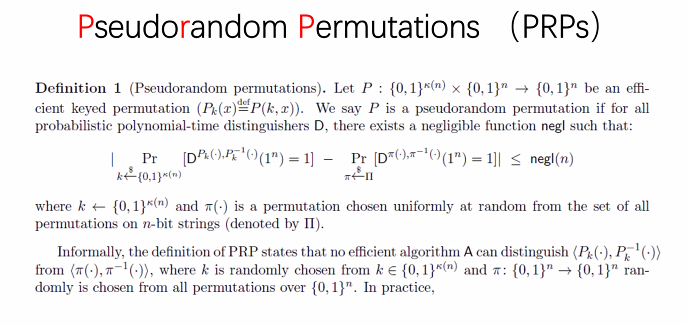
Figure 7: Definition of Pesuro-Random Permutation
This definition follows a common paradigm in cryptography: efficient approximation of ideal world from real world.
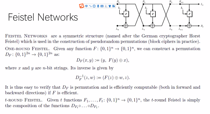
Figure 8: Feistel Networks: from PRF to PRP
The feature here is that both the permutation and its inverse are efficiently computable. And it can be easily concatenated.
The Luby-Rackoff PRP from PRF: four round construction.
Proof sketch. Seems like we can use RO-like argument for first four hybrids, in the final hybrid, i.e. using random function to implement a random permutation. It seems like birthday attack is unavoidable in this case.
What if we reduce the network to three rounds? This suffices for indistinguishability for only encryption oracle, rather than the evaluation oracle.
What about two rounds? If we first do a hash function \(h_1\) at the beginning and hash the two round output \(h_2\) after the end, we can do a PRP from two round Feistel.
Constructions of Block Ciphers
Ideal vs. Reality
In theory
One-way function (actually, we learned OWP, regular OWF, not any OWF) -> PRG -> PRF -> PRP
In practice
Built from scratch: AES / DES
A PRP can is a PRF up to a birthday bound
A PRP is at first, a PRF. In practice, PRP is acquired easily from AES. But permutation is a class more “structured” than random functions. So there is a gap (luckily not too big) between PRF and PRP.
Lemma. A (\(t\), \(\epsilon\), \(q\))-secure PRP on n-bits is a (\(t\), \(\epsilon + \frac{O(q^2)}{2^n}\), \(q\))-PRF.
Proof.
- Any (t, q)-Adv distinguishes PRP from RP with advantage \(\leq\epsilon\).
- Any (\(\infty\), q)-Adv distinguishes RP from RF with advantage \(O(q^{2}/2^{n})/\).
Mode of Operation
Direct use of a block cipher is not recommended. Message are a multiple of the cipher block size in length. The solution is different mode of operations.
- ECB (insecure)
- Cipher Block Chaining
- Cipher Feedback
- Output Feedback
- Counter (the difference from \(r, \prf_{k}( r) \oplus x\) is that CTR hash shorter ct, but is stateful)
Pseudoentropy and Pseudorandomness Extraction
Two types of Pseudoentropy.
- HILL pseudoentropy
- X has k bit HILL pentropy if it is indistinguishable in the non-uniform model from a k-bit unpredictable (unconditional) distribution.
- Metric-type pseudoentropy
- X has k bit Metrix type pseudoentropy if for every circuit D of size s there exists a distribution of at least k-bit min-entropy that is indistinghishable by \(D\) from \(X\).
Lecture 8
Pseudoentropy and pseudorandomness extraction.
Pseudoentropy
HILL and metric-type pesudoentropy.
- HILL pseudoentropy. We say \(X\) has HILL pseudoentropy \(k\) if there exists a distribution \(Y\) where \(\mathbf{H}_{\infty}(Y) \ge k\) and \(\mathsf{CD}(X, Y) \leq \epsilon\).
- Metric-type pseudoentropy. We say \(X\) has metric-type pseudoentropy \(k\) if for every circuit \(D\) of size \(s\) there exists a distribution \(Y\) with \(\mathbf{H}_{\infty}(Y) \ge k\) and \(\delta^D(X, Y) \le \epsilon\).
Borak proved 2 implies 1 using von Neumman’s Min-Max theorem. The idea is to prove after exchanging the quantifiers, the result is to some extent, equivalent.
Pseudoentropy of PRG conditioned on leakage
If \(\mathsf{PRG} : \{0,1\}^n \to \{0,1\}^m\) and \(f : \{0,1\}^n \to \{0,1\}^{\lambda}\)
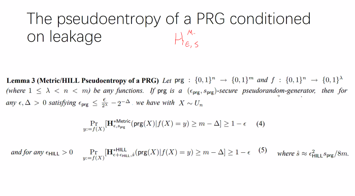
Figure 9: Peduroentropy of PRG
Without leakage, the pseudoentropy of PRG output is trivial. We want to prove similar result conditioned on arbitrary leakage.
Why do we use probability instead of plain assertion? The reason is that some leakage can be drastic. Using probability we can bypass this limitation. E.g. the leakage function \(f\) is the hamming weight of input. If we observed that \(f(x) = 0\), then it holds that \(x = 0\).
From the previous lemma 7, we only have to prove equation (4), which is a seemingly weaker (and hopefully easier to prove) result.
This lecture is based on a FOCS 2008 paper: Leakage Resilient Cryptography 这是一篇经典论文,贡献是
结论非常庞大,而且它试图通过理论的方法解决实际密码实现上的问题
证明过程中的一个结论是 Dense Model Theorem, 它与Green-Tao定理存在着联系
Green-Tao: 质数包含所有长度的等差数列,即给定\(\ell\),存在差为 \(\ell\)的素数等差数列
我们使用集合上的Dense Model Theorem。
Proof overview.
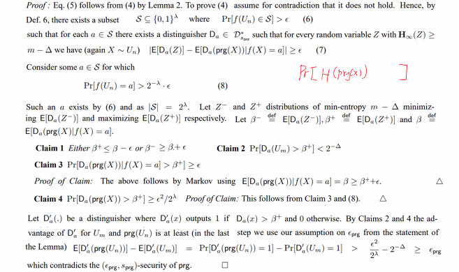
Figure 10: Simplified Proof
First consider the complement of the event, what we want to prove is …
One tricky part is that you can assume a 0-1 distinguisher can output one real number. This special type of distinguisher can be implied by standard distinguishers, by apprximating the probability \(\Pr[D=1]\).
Anyway, the proof showed that PRG is still secure under leakage. In particular, we have for a \(\mathsf{PRG}\), there exists a high-entropy \(Y\) such that \(\mathsf{PRG}(X), f(X)\) is indistinguishable from \(Y, f(Y)\). We can therefore use an extractor to extract randomness from \(Y | f(Y)\). This means that even for leaky source, we can extract randomness from PRG’s output using randomness extractor (e.g. universal hash function).
Non-Uniform Key wPRF
For a weak PRF, if we choose key to be slightly non-uniform, will the output still be pseudorandom?
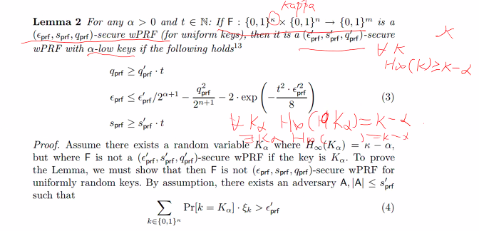
Figure 11: Non-uniform High-min-entropy Key in PRG Application
If you are interested, please refer to STOC 2008, EC 2009 (a simplified proof is presented in TCC 2013).
Exercises
Existence of Independent Code
Independent code: \(k\)-independent and \(k = n\) means that the code \(C\) is MDS code, which is trivial for \(\mathbb{F}_2\), so typically we have \(k < n\).
We relex the condition to proving a good enough probability over the choice of \(C\).
We first expand the probability in to summation over \(r\), and then observe that for random \(C\), since \(r\) is pair-wise disjoint, the r.v. \(Cr_1\) and \(Cr_2\) are independent for any \(r_1 \ne r_2\). Notice that altogether they are not independent (consider \(r_3 = r_1 + r_2\)). We can then use Chebyshev’s inequality to get the result.
One-Time MAC
Universal hash function
Collision Entropy and Min-Entropy Equivalence
Use Markov inequality.
PRG from LPN
One trick — flattening Shannon entropy. For \(H(w) = a\), we have \(\minentropy{w_1, w_2, \ldots, w_n} \approx na\). The definition-based conditional min-entorpy is somewhat pessimistic. The flattneing trick can be userful here.
Lecture 9
Exercise Solutions
PRG from LPN
First of all standard LPN with \(q = 2n\) and \(\mu = \frac{1}{4}\) implies Hermite normal form LPN’ where secret follows noise distribution \(Ber_{\mu}^n\).
So we first sample a \(4n\)-bit random number, and then through bitwise-AND, get a \(2n\)-bit random Bernoulli noise. Conditioned on this output, we still have whp. \(\frac{3n}{2} - \lambda\) 2-bit pairs that have \(\log 3\) entropy.
Procedure:
- First sample \(x, e\) from \(4n\)-bit uniform randomness.
- Then output \(A x + e\), and use randomness extractor to extract \(2n + \lambda\) bits.
Search-LPN and Decision-LPN
From Decision-LPN to Search-LPN: Compute \(x\) and accept iff. the hamming weight of \(y - Ax\) is small.
If input \(A, y\) follows LPN distribution, the algorithm will accept whp. If the input follows uniform distribution, then from the fact that
\[ \Pr_{A, y} [ \exists s, |y - As| \le \lambda ] \le 2^{ -m + n + \lambda \log(m) }, \]
we conclude that the probability the algorithm accept is bounded by the previous negligible probability.
From Search-LPN to Decision-LPN: There are at least three very related methods.
The first one is the most “orthodox” one. Construct hybrid \(H_0\), \(H_1\), \(\ldots\), \(H_q\). \(H_0\) is the LPN distribution, and \(H_q\) is the uniform distribution. Using GL theorem we can conclude from the one-wayness of LPN, changing \(a_i^T x\) to \(U_1\) is indistinguishable. So by hybrid argument we can conclude that \(H_0\) and \(H_q\) are indistinguishable.
Or we can follow the second way: using the LWE-like solver, solving the secret bit-by-bit.
Finally, we can use a very unorthodox method, without hybrid argument. Suppose there is a distinguisher that distinguishes LPN distribution and uniform distribution, then we can construct an algorithm that on input \(A, Ax+e, r\), output \(r^T, x\) with high probability. And from GL-theorem’s proof (the list decoding algorithm), this implies a solver for \(x\).
How to do that? First samples \(u \leftarrow \{0,1\}^q\), and then let \(\bar{A} = A - u\cdot r^T\). Observe that
\begin{align} A x + e &= (\bar{A} + u r^T) x + e \\ & = \bar{A} x + e + u (r^T x)\enspace. \end{align}
So when \(r^Tx = 0\), \(Ax + e\) follows LPN distribution with \(\bar{A}\) as public matrix, whereas when \(r^T x = 1\) output is random.
And thus \(\bar{A}, y = Ax+e\) follows
- LPN distribution when \(r^T x = 0\)
- Uniform distribution when \(r^T x = 1\)
This implies an effective distinguisher for the GL-hardcore.
Domain Extension
Conditioned on no collision at \(R_1\), the two distributions are identical. So we only have to bound the probability of collision. And the probability is just a birthday attack bound. As a matter of details, I think the probability should be computed as
\[ \Pr[\neg \text{Collision}] \ge (1) (1 - \frac{1}{2^l}) (1 - \frac{2}{2^l})\ldots (1 - \frac{q-1}{2^l}) = 1 - O(\frac{q^2}{2^{l+1}})\enspace, \]
whereas I am not sure how to formulate the \(\binom{q}{2}\)-pair bound, since collision can occur at each level.
One tricky part is that after query, the hash function \(h\) can be made public. So the attack can be made a two-stage process. First the attacker is given oracle access to a PRF (\(R^{\prime} = R \circ H\)), and in the second stage, the attacker is given the transcript of the attack, along with the hash function. This is clearly a relaxation, but does not affect security.
CRHF and UOWHF
U(OW)HF is an one-way version of UHF. CRHF is considered to be the strongest primitive in symmetric cryptography, although no black-box construction based on OWF exists.
Collision Resistance Hash Function
CRHF is a family of Hash funcitons such that:
- Efficient
- polynomial computable sampling and evaluation algorithms
- Shrinking
- opposite to stretching
- Collision Resistant
- given random instance, any PPT adversary cannot find a collision
\[ \Pr_{g\leftarrow G; (x, x^{\prime}) \gets A(1^n, g)} [x\ne x^{\prime}\land g(x) = g(x^{\prime})] = \mathsf{negl} \]
Birthday attack. Use \(2^{\frac{m}{2}}\) time to find from \(2^m\)-output domain a collision with a constant probability (since the collision probability with random output among \(2^m\) and \(q\) queries is \(\Theta(\frac{q^2}{2^m})\)). This implies that any CRHF with output size \(m\) has security no more than \(\frac{m}{2}\).
Practical examples:
- MD5
- output 128bits, broken
- SHA1
- output 160bits, broken
- SHA256
- output 256bits, unlikely to break
Theoretically black-box construction of CRHF based on OWF is impossible.
Universal One-Way Hash Function
UOWHF is a family of Hash funcitons such that:
- Efficient
- polynomial computable sampling and computing
- Shrinking
- opposite to stretching
- Target Collision Resistant
- given random instance, a target, any PPT adversary cannot find a collision. For any \(x\in \{0,1\}^n\),
\[ \Pr_{g\leftarrow G; x^{\prime}\gets A(1^n, g,x))} [x\ne x^{\prime}\land g(x) = g(x^{\prime})] = \mathsf{negl}. \]
TCR limits the form of collison (by setting a “target”), so it is a weaker version of CR.
TCR is equivalent to another notion called TCR2. In this definition, the target \(x\) is chosen uniformly at random. That TCR implies TCR2 is trivial, while in the opposite direction, we can construct a TCR hash from a TCR2 hash, by adding \(n\)-bit to function description, and xoring \(a\) with input before every evaluation. That is, \(g^{\prime}(x) = g(x \oplus a)\).
The reduction is trivial. Suppose there exists a target \(a\) that allows an algorithm \(A\) finds collision with non-negligible probability, then we can first ask TCR2 challenger for a hash function \(g\) and target \(x\), then send to algorithm \(A\) \(g_{x \oplus a}\) and \(a\). If such a collision \(b\) is found, it holds that \(g(x) = g(x \oplus a \oplus b)\).
UOWHF is good enough for digital signatures, and it is implied from OWF. This concept, together with a reduction from OWP, was presented by Naor and Yung.
UOWHF can be seen as dual to PRG.
UOWHF from OWP
Let \(f: \{0,1\}^n \to \{0,1\}^n\) be any (\(t\), \(\epsilon\))-one-way permutation, and \(H\) be a family of universal hash permutations over \(\{0,1\}^n\),
\[ H = \{ h:\{0,1\}^n \to \{0,1\}^{n} | h(y) := h\cdot y, h\ne {\bf 0}, y\in GF(2^n) \}\enspace, \]
let \(\mathsf{trunc}\) be the function that truncates the last bit of its \(n\)-bit input. Then we argue that
\[G := \{ (\mathsf{trunc} \circ h \circ f) | h\in H \}\]
is a family of (\(t - n^{O(1)}\), \(\epsilon\)) UOWHF with 1bit shrinkage.
Proof
We can construct an inversion algorithm for OWP based on Collision finder of TCR2. The key is that we can “program” the hash function in the middle to meet our need.
Given input \(y\), we first samples \(x^{\prime} \leftarrow \{0,1\}^n\). With probability \(\frac{1}{2^n}\) we can success at this step (\(f(x^{\prime} = y\)). If not, we continue by computing \(h = (00\ldots 01)\cdot (y - x^{\prime})^{-1}\). Notice that this implies
\[ \mathsf{trunc} \circ h \circ \underbrace{f (x)}_{y} = \mathsf{trunc} \circ h \circ f (x^{\prime})\enspace, \]
and since \(x^{\prime} \) and \(x\) are iid, \(h\) is indeed random. If the inversion algorithm has probability \(\epsilon\) when the input is \(h, x^{\prime}\), then with the same probability we can find \(x\) since the hash function is \(2\)-regular. Altogether, we obtain a OWP inverter that succeed with at least \(\epsilon\) probability.
Merkle-Damgard Domain Extension for CRHFs and UOWHFs
Let
\[G \subseteq \{ g: \{0,1\}^n \to \{0,1\}^{n-s} \} \]
for each \(g : (x_i,r_i) \to x_{i+1}\), where \(x_i, x_{i+1} \in \{0,1\}^{n-s}\), \(r_i \in \{0,1\}^s\), be a (\(t\), \(\epsilon\))-secure CRHF, and for any \(q \in \mathbb{N}\) define \(G^q \subseteq \{0,1\}^{n + (q-1) s} \to \{0,1\}^{n-s}, g\in G\) where
\[ g^q(x_{1}, r_1, r_2, \ldots, r_q) = g(\ldots g(g(x_1, r_1), r_2), \ldots, r_q). \]
Then we have (\(t - q t_g\), \(\epsilon\))-CRHF.
Proof
From the “bigger” collision we can find a smaller collison at the \(i^{th}\) level such that \(g(x_i, r_i) = g(x^{\prime}_i, r^{\prime}_i)\) and \((x_i, r_i) \ne (x_i^{\prime}, r_i^{\prime})\). And that contradicts the assumption that \(g\) is CRHF. The time loss is incurred at the checking step.
Merkle-Damgard Domain Extension for UOWHFs.
Let
\[ G \subseteq \{ g: \{0,1\}^n \to \{0,1\}^{n-s} \} \]
for each \(g : (x_i,r_i) \to x_{i+1}\), where \(x_i, x_{i+1} \in \{0,1\}^{n-s}\), \(r_i \in \{0,1\}^s\), be a (\(t\), \(\epsilon\))-secure UOWHF, and for any \(q \in \mathbb{N}\) define \(G^q \subseteq \{0,1\}^{n + (q-1) s} \to \{0,1\}^{n-s}\), \(g_{1}, g_2, \ldots, g_q \in G\) where
\[ g^q(x_{1}, r_1, r_2, \ldots, r_q) = g_q(\ldots g_2(g_1(x_1, r_1), r_2), \ldots, r_q)\enspace. \]
Then we have (\(t - q t_g\), \(q \epsilon \))-UOWHF.
Proof
This proof is somewhat tricker than the previous proof, since we have to embed the target into it. Using the TCR (instead of TCR2) definition, we can settle with arguing existential property, but throughout the proof one must beware that the target \(y\) must be independent of the UOWHF function (this is probabilty the reason behind \(q\)-many independent hash functions in the definition).
Suppose through contradiction, there exists an algorithm running in \(t - qt_g\)-time and a target \(y = (x_1, r_1, \ldots, r_q)\) such that
\[ \Pr_{g_1,g_2,\ldots,g_q \leftarrow G; y^{\prime} \gets A(y, g_1, \ldots, g_q)} [y \ne y^{\prime} \land g^q(y) = g^q(y^{\prime})] \ge q\epsilon\enspace, \]
We can find a \(t\)-time algorithm \(A^{\prime}\) and target \((x_i^{\star}, r_i^{\star})\) finds with at least \(\epsilon\)-probability. First consider a random index \(i^{\star} \leftarrow [q]\), random hash functions \(g_1, \ldots, g_{i^{\star} - 1} \leftarrow G\), and define \(x_i^{\star}, r_i^{\star} = g^{i^{\star} - 1} (x_1, r_1, \ldots, r_{i^{\star} - 1})\). Now we let \(g_{i^{\star}} = g\) which is the algorithm \(A^{\prime}\)’s input, and sample the rest hash functions at random.
By the assumption, since our definition of \(q\) hash functions follows the uniform distribution over \(G^q\), with probability \(q\epsilon\) the algorithm \(A\) will return a collison \(y^{\prime}\). And since the index \(i^{\star}\) is independent with \(A\)’s input, with probability at least \(\frac{1}{q}\), the collision will occur at position \(i^{\star}\). Id est, we can get \(x_{i^{\star}}^{\prime}, r_{i^{\star}}^{\prime}\) that constitutes a collision for the hash function \(g\). Formally, we have
\begin{align*} & \Pr_{ i^{\star} \leftarrow [q]; g \leftarrow G; (x^{\prime}_{i^{\star}}, r^{\prime}_{i^{\star}}) \gets A(x_{i^{\star}}, r_{i^{\star}}) } [(x^{\prime}_{i^{\star}}, r^{\prime}_{i^{\star}}) \neq (x_{i^{\star}}, r_{i^{\star}}) \land g(x_{i^{\star}}, r_{i^{\star}}) = g(x^{\prime}_{i^{\star}}, r^{\prime}_{i^{\star}})] \\ & \ge \Pr_{\vec{g} \leftarrow G^q; y^{\prime} \leftarrow A^{\prime}(\vec{g})} [y \ne y^{\prime} \land g^q(y) = g^q(y^{\prime})] \cdot \Pr_{i^{\star} \leftarrow [q]} [i = i^{\star}] \\ & \ge q\epsilon \cdot \frac{1}{q} \\ & = \epsilon\enspace. \end{align*}
Finally, since in the above argument, the target \(x_{i^{\star}}, r_{i^{\star}}\) only depends on \(y\) and random choice of \(i^{\star}\) and \(g_1, g_2, \ldots, g_{i^{\star} - 1}\), we conclude by average argument there exists one specific target that has more than ε advantage.
Remarks
It seems that if we use only one hash function in the construction, the target throughout the argument will be dependent on the hash function itself, rendering the final averaing argument invalid. It is definitely an obstacle, whether or not its an artifact I currently have no idea.
Merkle-Damgard Tree — More Efficient Domain Extension
If we have a length-halving function, then we can use an “inverse” GGM tree. One caveat is that this tree has depth \(O(\log n)\) whereas GGM has linear depth.
Lecture 10
Continuing on hash functions
CRHF is a very natural definition, but no black-box construction based on OWF of CRHF seems possible. UOWHF has a weaker definition, but still strong enough to support many applications, including:
- Digital signatures
- Cramer-Shoup PKE scheme
- Statistical hiding commitment
It should be noted that both UOWHFs and CRHFs are families of functions, rather than a single one.
We have a simple, effective generic construction based on OWP and UHF. Quite like the complimentary to the OWP based stretch-1 PRG construction.
Domain extension, in the inverse direction.
In the tree-like construction for UOWHF, one still have to use different functions in different layers. Though there has not been any proof against using the same hash function every layer, doing so would render the regular proof invalid, since we have to embed a target (either some target in the TCR definition or a random target in the TCR2 definition) into the challenge target, this target has to be independent with the instance \(g\).
Specifically, if we use the instance \(g\) in every layer of the challenge instance, there is a (seemingly) inherent correlation between \(g\) and the challenge target \(t^{*}\). On the other hand, if we use independent hashes every layer, we can guess one instance \(i^{\star}\) and embed the input hash instance \(g\) into that layer. In this case, success happens when the output collision position coincides with our guess, and the collision target now will only depend on \(y\) and random choice independent of \(g\). An averaging argument can then be applied to argue the existence of some valid target.
Extension to UOWHF
(Almost) Optimal Constructions of UOWHFs from 1-to-1, Regular One way Functions and Beyond.
As Prof. Lai pointed out, in some decsipline, 1-to-1 means bijective. So to clearify the notation, the term “1-to-1” means injective in this lecture.
CHRFs are UOWHFs, but OWFs imply UOWHFs but not CRHFs.
Symmetric Crypto Hierarchy
| Many Crypto Applications | ||
| PRF | Digital Signature | Stat ZK |
| PRG | UOWHFs [NY89,HHRVW10] | Stat Hiding Com. |
| One Way Functions | ||
Duality Between PRGs and UOWHFs
From length-\(n\) OWF, we can have PRG with input length \(\tilde{O}(n^3)\). Or UOWHF with output length \(\tilde{O}(n^7)\).
It seems like the PRG line is already pushed to the limit. In an annecdote, Yu met with Zheng (a la [YZ12]) in a 2013 meeting, where Zheng informed him after this work with PRG, he decided to ditch theory and instead work in industry (Google).
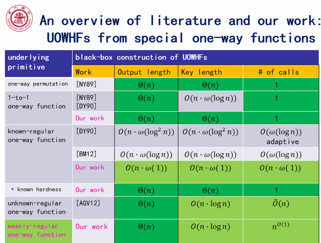
Figure 12: Overview of this work
Universal Hashing
UHF from finite group multiplication and truncating.
Well-known hashing properties:
- Leftover hash lemma
- For any \(X\in\{0,1\}^n\) with \(\mathbf{H}_{\infty}(X) \ge m + d\), conditioned on \(h \leftarrow H\), \(h(X)\) is \(2^{-\frac{d}{2}}\)-close to uniform.
- Injective hash lemma
- For any \(X \in \{0,1\}^n\) with \(H_0(X) \le m - d\), we have \(\Pr_{h\leftarrow H, x\leftarrow X}[ \exists x^{\prime} \ne x: h(x) = h(x^{\prime} ] \le 2^{-\Omega(d)}\). This can be proved using a simple union bound on \(x^{\prime}\).
Original UOWHFs from OWP
Assumption
(\(t\), ε)-one-way permutation \(f : \{0,1\}^n \to \{0,1\}^n\). We use a UHF family \(H\) and a truncating function \(\mathsf{trunc} : \{0,1\}^n \to \{0,1\}^{n-s} \).
Statement
\(G : \{ \mathsf{trunc} \circ h \circ f : h \in H\}\) is a family of (\(t - n^{O(1)}\), \(2^s \epsilon\))-secure UOWHFs.
Proof
We can adapt the proof for the original 1-bit shrinkage construction to this case. First we make a guess \(x \leftarrow \{0,1\}^n\) and returns if the guess is correct. Or else, we guess \(v = 0\ldots0\bar{v}, \bar{v} \leftarrow \{0,1\}^s\) and compute \(h = (y^{*} - f(x))^{-1} v\). After that, we send \(g = \mathsf{trunc} \circ h \circ f\) and \(x\) to \(A\) and receives its result \(x^{\prime}\). Notice that we have \( h \cdot (f(x) - f(x^{\prime}) \ne 0\). So if it happens that the choice of \(v\) makes this \(x^{\prime}\) the preimage of \(y^{*}\) with probability \(\frac{1}{2^s - 1}\).
Original UOWHFs from 1-to-1 OWFs
Assumption
(\(t\), \(\epsilon\))-1-to-1 OWF \(f : \{0,1\}^n \to \{0,1\}^l\) ((\(l > n\))
Tools
UHF \(H_0\), \(\ldots\), \(H_{l - n}\), where \(H_i : \{ h_i : \{0,1\}^{l-i} \to \{0,1\}^{l-i-1}\}\).
Statement
\(G : \{h_{l-n} \circ \ldots \circ h_0 \circ f\}\) is a family of (\(t - n^{O(1)}\), \(\epsilon\))-UOWHFs.
Use \(l - n + 1\) independent hash functions to shrink \(f(x)\) where \(f : \{0,1\}^n \to \{0,1\}^l\) is a OWF. But the excessive use of hash function seems to be an artifact of its proof. But right now I have yet found out how to prove it.
Construction 1: UOWHFs from 1-to-1 OWFs
Assumption
(t, ε)-1-to-1 OWF \(f: \{0,1\}^n \to \{0,1\}^l\) ( \(l > n\) ).
Tool
Universal hash function \(H = \{ h: \{0,1\}^l \to \{0,1\}^l\} \), Truncating function \(\mathsf{trunc} : \{0,1\}^l \to \{0,1\}^{n-s}\)
Statement
\(G : \{ \mathsf{trunc} \circ h \circ f : h\in H\} \) is a family of (\(t - n^{O(1)}\), \(2^{s+1} \epsilon\))-UOWHFs.
Proof
We can use an alternative definition of OWF, taking account of the fact that \(f\)’s range is sparse.
Construction 2
Skipped.
CRHF from LPN
Russell Impagliazzo’s Complexity Worlds
- Algorithmica
- \(\mathcal{P} = \mathcal{NP}\) (or \(\mathcal{NP} \subseteq \mathcal{BPP}\))
- Heuristica
- \(\mathcal{NP} \ne \mathcal{P}\) but \((\mathcal{NP}, \mathcal{U}) \subseteq \mathcal{AvgP}\); \(\mathcal{NP} \not\subseteq \mathcal{BPP}\) but \((\mathcal{NP}, \mathcal{U}) \subseteq \mathcal{HeurBPP}\)
- Pessiland
- \(\mathcal{NP}, \mathcal{PSamp} \not\subseteq \mathcal{HeurBPP}\), but \(\not\exists \mathsf{OWF}\))
- Minicrypt
- \(\exists\) one way function ( 单向函数 ) but \(\not\exists\) public key crypto( 公钥密码)
- Cryptomania
- \(\exists\) public key crypto ( 公钥密码 ) & multiparty computation 安全多方计算
- Obfustopia
- \(\exists\) fully homomorphic encryption ( 全同态加密) & obfuscation 混淆
\(\mathcal{NP}\) vs. OWF
\(\mathcal{NP}\) problem: easy to verify. \(\mathcal{NP}\)-hardness is defined via reduction. Its conjectured however, that \mathcal{NP} is superpolynomially hard.
LPN Problem
It seems like that Learning with Error, Nearest Codeword Problem, Learning Parity with Noise are all related.
With smoothing lemma, we can prove the reduction from worst-case NCP to average-case LPN.
Overview of the reduction
Consider the a NCP instance \(A, c = Ax + e\), we want to randomize it by multiplying a matrix \(B\) and randomizing the secret accordingly. So we sample \(x^{\prime}\) at random and comput \(BA\), and \(Bc + BAx^{\prime} = BA (x + x^{\prime}) + B e\). To ensure low noise, we have to make \(B\) sparse. The smoothing lemma states that for A that corresponds to balanced code, if \(B \gets Ber_{\mu}^{q \times m}\) we have
\[ (BA, Be) \approx_s (U^{q \times n}, Ber_{\mu}^q). \]
There is however a simpler proof using Vazirani’s XOR lemma, that I have proof read but have yet finished. I have already read Vazirani’s XOR lemma, perhaps I should read it.
Hardness of NCP and LPN
It seems that worst case NCP has time complexity \(\mathsf{poly}(n) \cdot e^{\mu n}\). For average LPN, the BKW algorithm gives \(2^{O(\frac{n}{\log n})}\) complexity. So it seems that worst case NCP is indeed very hard.
Cryptographic Hashing from LPN
Construct a intermediate problem \(\mathsf{bSVP}\) that is the analogue to SIS problem. We then construct an Expand function that is
- 1-to-1
- output sparse 0-1 vector
- parallel
We can then directly get a CRHF.
Expand
The expand function is very easy. For \(L\cdot t\) bit input, the function expand it to \(2^L \cdot t\) bit output, by first partition the input into \(t\) \(L\)-bit blocks, translate each block into “one-hot” encoding, and then output. The output has exactly \(t\) ones, and by definition it is an injective map.
LPN Implies bSVP
Suppose we have a bSVP solver \(O\), we can construct a distringuisher \(A^O(A, y)\).
We can first find a solution \(x\) to \(A^T\), them determine which is the case by the bias of \(y^Tx\). If \(y\) is uniform, then \(y^Tx\) is also uniformly random. Otherwise, \(y^Tx\) has biased Bernoulli distribution from piling up lemma.
This reminds me of knapsack LPN problem.
Hardness
T-hard (\(n\), \(\mu\), \(m\))-LPN implies \(\sqrt{T}\)-hard CRH \(h_A\), where \(h_A (y) = A \cdot \mathsf{Expand}(y)\), \(t^2 \le m \le T = 2^{\frac{\mu t}{1 - 2\mu}}\).
I wonder if Knapsack-LPN can be used to construct a CRHF and how this theorem is proved.
Overcoming Weak Expectations
Typical crypto setting \(P\): pick random secret key \(R \leftarrow \{0,1\}^m\). But in practice, we can only guarantee that \(R\) has large entropy.
There are three options. (\(X\) is the weak source)
- Clever
- Design \(P\) so that it can withstand weak randomness
- Modular
- Design key deriviation function \(h : \{0,1\}^n \to \{0,1\}^m\) subject to \(R = h(X)\) is good for \(P\). The goal is to assume little-to-nothing about \(P\).
- Dumb
- Use \(R = X\) and hope for the best.
Pedantic Viewpoint
Fix \(P\) and any “legal” \(A\) Let \(f( r)\) be the advantage of \(A\) on key \(r\).
- Unpredictability apps: \(f( r) \in [0,1]\)
- Indistinguishability apps: \(f( r) \in [-\frac{1}{2}, \frac{1}{2}]\)
- In the ideal world, the advantage of \(A\) is \(|E(f(U_m))| = |\sum_r \frac{1}{2^m} f( r)|\)
- In the real world, the advantage of \(A\) is \(|E(f( R))| = |\sum_r p( r) \cdot f( r) |\)
Simple Case
For unpredictability application, we have any (\(t\), \(\epsilon\))-secure \(P\) in the ideal model is also (\(t\), \(\ 2^d \cdot epsilon\))-secure in the \(m-d\)-real model.
Proof
\(E_r(p( r)\cdot f( r)) \le 2^m \frac{1}{2^{m-d}} \sum_r \frac{1}{2^m} f( r) = 2^d E(f(U_m))\).
Notice that we used the fact \(f( r)\) is non-negative throughout the proof.
Indistinguishablility Application
The paper introduced a square security notation, but I have yet grasped it.
Lecture 11
From this lecture through the next three or four lectures, Prof. Liu will take on this lecture. 两节课讲一下现代密码学的主要原则,然后在之后讲IBE,ABE,FHE等内容,再讲一两个证明。
Outline
- A brief introduction
- Principles of Modern Crypto
- framework of modern crypto
- mathematics of pkc
- PKE
- Digital signature
- Hash function
- Hybrid encryption and PKE
A Brief Introduction to Crypto
Crypto ≈ Cryptography + Cryptanalysis
Usually cryptanalysis is very important in symmetric-key cryptography (e.g. Hash function, secret-key cryptography).
The Basis Goals of Cryptography
- Enabling parties to communicate over an open communiation channel in a secure (confidentiality, integrity) way.
- Cryptogrpahic primintives
- Secrecy / Confidentiality: SKE / PKE
- Integrity / Authenticity: MAC / PKE, using Hash Function (this primitive is keyless, isn’t there public coins?)
Private Key Encryption
Two parties share keys previously.
Message Authentication Code
Only sender and receiver can compute and verify MAC.
Public Key Cryptography
Modern provable security is (arguably) more biased towards PKC.
In pure symmetric crypto, people typically use a centralized online key distribution server to handle session key establishment requests. Whereas in public key setting, one can use certificates to do this.
In 1976, W. Diffie and M. Hellman purposed a paper “New Directions in Cryptography” to motivate simplifaction of key distribution and management in symmetric-key cryptography.
Digital Signature
Like MAC, but publicly verifiable.
- Public Verifiability
- Transferability
- Non-repudiation
Principles and Framework of Modern Cryptography
Classic cryptography — symmetric key encryption algorithms.
- Classical Cryptography
- Art
- Ad-hoc
- Modern Cryptography (Methodological)
- Science
- Components
- Syntax (what components should a system have)
- Security Models (what is the definition of security and what is the adversary’s ability)
- Provable Security (reduction)
Private Key Encryption
Syntax: three algorithms
- \(KeyGen(1^n) \to k\)
- \(Enc(k, m) \to c\)
- \(Dec(k, c) \to m\)
We can then define key space \(\mathcal{K}\), messsage space \(\mathcal{m}\) and correctness of private-key encryption.
Key space for single-table substitution: \(26!\)
Kerckhoff’s Principle
Security only depends on secrecy of key, rather than the algorithm. The rationale behind this principle is that changing keys is much easier than changing algorithms. So to be more complete, cryptographic designs should be made completely public.
Moreover, it feels safer after witnessing every one around the globe failed to break a published cryptographic scheme.
So It appears there are indeed people who believe that algorithms should be kept secret (at least in the civilian application).
Brute-Force
At least the key space should be large enough to make exhaust-search attack infeasible. But note that this is not sufficient.
Principles of Modern Cryptography
Principle 1
Formal Definitions, provides what threats are in scope and what security guarantees are desired. Security guarantee and threat model.
- Security gurantee — semantic security, not a bit of additional information is leaked
- Threat model — Ciphertext-only attack, known-plaintext attack, chosen-plaintext attack, chosen-ciphertext attack.
Lecture 12
现代密码学的原则
- 明确定义
- 包括正确性、安全性的定义(threat model, security guarantee)
- 精确的假设
- 由于需要使用计算安全性,而统计意义上的安全性很难得到 We are almost entirely talked away from using ad hoc assumptions. Though this principle has nothing to do with the content of assumptions.
- 安全性证明
- 定义与假设允许我们分析,安全保证能否在相应的模型下被假设蕴含,这就是安全性证明的功能
Provable Security and Real-World Security
The art part of modern cryptography: rigorous approach leaves room for creativity in:
- Developing definitions suited to contemporary applications and environments (e.g. CCA, UC)
- Proposing new mathematical assumptions (e.g. Coppersmith, Shor)
- Designing new primitives (e.g. IBE a la Shamir, PKE a la Diffie and Hellman)
- Constructing novel schemes and proving them secure
- Attacking deployed cryptosystems
Provable Security and Real-World Security
A proof of security is always relative to the definition being considered and the assumptions being used.
The proof may be irrelevant if
- The security guarantee does not match what is needed
- The threat model does not capture the adversary’s ture abilities
The proof of security is meaningless if the assumption is refuted.
Framework of Modern Cryptography
Personal summary of Prof. Liu. Framework
- Symmetric Cryptography
- Encryption
- Message Authentication Code
- Asymmetric Cryptography
- Public Key Encryption
- Digital Signature
- IBE, ABE, FHE
- Blind Signature, Ring Signature
- Commitment, Zero-Knowledge Proof
- Hash function
Research Directions in Asymmetric Cryptogrpahy
- 应用密码算法的业务系统
- 应用密码算法的协议
- 密码原语的定义:应用驱动、密码理论研究
- 密码原语方案设计:构造符合源于定义并在其模型下证明安全的方案
- 困难设计:困难问题的求解算法研究
Number Theory
Cyclic Group
Primes
Generating large primes — a probablistic method. Sample a random large enough number, using a conjecture we can argue that with large probability we can actually get a prime number, if we repeat the process a small number of times. The primality test can be a coRP algorithm.
Discrete Logarithm Assumption
We always work on finite groups. The groupgen algorithm generates algorithms for “translation” in \(\mathbb{G}\). Theoretically, a GroupGen algorithm is related to the instance of DL, CDH, DDH instance, but in practice we can simply choose NIST recommended standard values.
An Example GenGroup Algorithm
- Generate a uniform n-bit prime \(q\)
- Choose a \(l\)-bit prime \(p\) such that \(q | (p - 1)\)
- Choose a uniform \(h \leftarrow \mathbb{Z}_p^{*}\)
- Set \(g = h^{\frac{p - 1}{q}}\)
- Output \(g, q, p\)
Another GenGroup Algorithm
- On subgroups of finite field
- On Elliptic Curves (cf. ECDSA)
Inverse on a Generic Group
Simply \(h^{-1} = h^{q - 1}\).
Public Key Cryptography
CPA / CCA threat model and IND / SS security guarantee.
Trick: if the fine-defined constraint, e.g. challenge ciphertext cannot be further queried, is not used, then the proof itself is most certainly useless.
Lecture 13
Some kind of code: 787228. Last lecture we have covered public key encryption. This lecture we will continue with digital signature.
Digital Signature
Patches need to be verified publicly.
Properties:
Correctness. \(\mathsf{Verify} (pk, m, \mathsf{Sign} (sk, m)) = 1\) for every \(m\)
Security (EUF).
- Security guarantee: non-forgeability
- Threat model: signing oracle, the advantage is just the success probability of forgery.
Extension: strong unforgeability, which means challenge (\(m\), \(\sigma\)) pair needs to be unique, rather than \(m\) has to be unique.
Example
DSA and *ECDSA both are included in the current Digital Signature Standard, issued by NIST.
Although ECDSA is no longer the recommended DS standard, it is still considered more efficient and have at least the same security level as RSA signatures. In ECDSA, the group parameter can be shared, whereas in RSA the encryption modulus cannot be shared.
Syntax: A group generation algorithm that generates the description of a cyclic group, its order and a generator. An example is to generate the prime-\(q\)-order subgroup of a larger multiplicative group \(\mathbb{Z}_p^{*}\).
- \(KeyGen(1^n) \to (pk, sk)\)
The group parameter can be considered public. In practice, this algorithm can just sample a private order and output \(pk = \mbox{group}, g^x\) and \(sk = x\).
Also, two functions \(H: \{0,1\}^{*} \to \mathbb{Z}_q\) and \(F: \mathbb{G} \to \mathbb{Z}_q\) are included in the public key as auxiliary information.
- \(\mathsf{Sign}(sk, m) \to c\) First hash the message to \(\mu = H(m) \), and then sample \(k \leftarrow \mathbb{Z}_q\). Then compute \(r =F(g^k) \), and \(s = k^{-1} (\mu + xr)\). If \(r = 0\) or \(s = 0\), sample \(k\) again and repeat. Output \(\sigma = (r, s)\).
- \(\verify(pk, m, \sigma) \to \{0,1\}\) Output 1 iff. \(r = F(g^{H(m) s^{-1}} y^{r s^{-1}})\).
Security: to prove the euf-cma security of DSA / ECDSA, the function \(F, H\) should be modelled as random oracle. \(H\) can sometimes be considered as a random oracle, \(F\) is completely not like a hash function. In DSA, \(F\) is just modulo \(q\); In ECDSA, \(F\) is the first coordinate modulo \(q\).
Hash Function
Syntax: \(H: \{0,1\}^n \to \{0,1\}^{l(n)}\).
Security guarantee: collision-resistant.
Weaker Security: second-preimage or target-collision resistance: given a uniform \(x\) it is infeasible to find \(x^{\prime}\) such that \(x\) and \(x^{\prime}\) collides.
Preimage resistance: given a uniform target \(y\) it is infeasible to find \(x\) such that \(y = H(x)\).
Birthday attack: an upper bound on the security of \(l(n)\)-long is \(l(n) / 2\).
Popular Crypto Hashes:
- MD5
- Broken
- SHA1
- Nearly broken
- SHA2
- OK
- SHA3
- Secure but slow
Hybrid Encryption
Encapsulate a symmetric session key from public key encryption, and then use this session key to encrypt subsequent data.
KEM / DEM are a new pair of primitives to capture / simplify hybrid encryption method.
Key Encapsulation Method
Syntax: there are three algorithms \(KeyGen\), \(Encap\), \(Decap\)
The CPA security is defined as follows. The challenge text is a ciphertext and a key. If \(b = 0\), the ciphertext is the encryption of the key; if \(k = 1\), the key and the ciphertext are independent. The adversary guesses the value \(b\).
The CCA security is defined by adding a decryption oracle.
Example
El Gamal-like KEM: actually I think it is more like DH-key exchange. Up on agreeing \(g^{xy}\), both sides hash this value to produce a key.
Lecture 14
Introduction to IBE
Starting from motivation (i.e. application in real life), abstract the definition.
From definition derive a construction and the security threat model.
From security model and construction, derive a security proof.
Motivation of Idenity-based Encryption
Public key cryptogrpahy partly solved the key distribution nuisance in symmetric key cryptography, but PKI is still somewhat troublesome. So key distribution should not be considered completely solved in PKC.
Introduction to IBE
Certification issuing is not free.
Adi Shamir introduced IBE in 1984. The application scenario is one-time key distribution in a large system (e.g. bank and multinational corporation).
One generalization is that an arbitrary string can be used as the public key.
The concept of Identity-based Cryptography
- Introduced by A. Shamir in 1984
- Identity-based Signature Scheme was proposed in 1987
- The first usable identity-based encryption shcemes were purposed in 2001 from pairing and QR
Correctness
If the same \(id\) is used, decryption will ensure plaintext recovery.
Security
IND-ID-CCA: Define two oracles
- \(OKeyGen(id) \mapsto KeyGen(mpk, msk, id)\)
- \(ODec(id, ct) \mapsto Dec(mpk, KeyGen(mpk, msk, id), ct)\)
And a number of restrictions:
- The challenge identity must not be previously queried to \(OKeyGen\)
- After challenge phase, the adversary must not query \(OKeyGen\) with \(id^{\star}\) or query \(ODec\) with \(id^{\star}, c^{\star}\).
Construction
Underlying Mathematics
Bilinear Map Groups: Let \(G\) and \(G_T\) be two cyclic groups of order \(p\) and \(q\), then a map \(e: G \times G \mapsto G_T\) is a bilinear map if
- Bilinear
- for all \(u, v \in G\) and \(a, b \in \mathbb{Z}\) it holds that \(e(u^a, v^b) = e(u, v)^{ab}\).
- Non-degenerate
- \(e (g, g) \ne q_{G_T}\).
We say \(G\) is a bilinear group if the group operation in \(G\) can be computed efficiently and there exists a group \(G_T\) and an efficiently computable bilinear map \(e: G \times G \to G_T\) as above.
We let \(GenGroup\) a group generation algorithm that generates \(G, G_T, p, q, e\).
BDH assumption: It is hard to compute \(e(g, g)^{abc}\) given random \(g, g^a, g^b, g^c\).
Original Construciton
The original construction satisfies IND-ID-CCA security in the RO model. Some considered selective IND-sID-CCA security in the standard model.
A number of subsequent works improved the security.
Further Development
The PKG can read any ciphertexts. This can introduce
- key escrow problem
- The revocation of user secret keys
- Anonymous IBE (Homework)
- Hierarchical IBE
Digital Signature
ECDSA is the key algorithm to ensure Bitcoin’s functionality.
In Bitcoin, transaction is authenticated by ECDSA. A wallet is the database of pk / sk pairs. In Bitcoin and other cryptocurrency, it is a desireable thing to have deterministic wallets.
Advantages of Deterministic Wallet
- Low-maintenance wallets with easy backup and recovery (just backup the seed)
- Freshly generated cold addresses (cold means never been on the Internet)
- Trustless audit
- Hierarchical wallet allowing a treasurer to allocate funds to departments
Though it should be noted that the treasurer use case and auditor use case cannot be used together.
Stealth address and determinstic wallet.
Lecture 15
Deterministic Wallet
Cryptographically, not very sound.
Wallet vs. Stealth Address
Wallet: managing the keys from the wallet owner.
Stealth address: to send money to a certain publicly visible master key in such a way that this key does not appear in the ledger at all, so that users’ privacy gets more protection.
Stealth address can serve as wallet, as a matter of fact.
Monero
| The Payer | The public | The Payee |
|---|---|---|
| A = aG, B = bG | \((a,b)\in\mathbb{Z}_p^2\) | |
| \(r\leftarrow \mathbb{Z}_p\) | \(R = rG\) | \(s = H(aR) + b\) |
| \(S = H(rA)G + B\) |
For each transaction, the payer uses a different \(r\).
Properties (intuitive)
- Privacy
- Each coin receiving address is freshly generated, with random \(r\)
- Security
- Only the payee knows \(b\)
- Convenience
- The check needs to be run each for each transaction
- Enhanced Security and Convenience
- \(b\) can be stored in cold storage
- Can be used to implement trustless audit.
Problem
If one secret key is compromised, the master secret key may be compromised.
Rationale of the Problem
Functionality
- User has a Master Public Key
- Payer can compute a DVK from MPK without interaction
- User can examine from DVK if its the recepient
Correctness
Checking transaction and signature verification algorithms are both correct
Unforgeability
Three oracles: verification key adding oracle, signing key corruption oracle, and signing oracle.
Notice that signing key corruption orecle, designed to take care of signing key corruption, is not considered in Monero. That is way Monero has the aforementioned problem.
Commitment Schemes
This part is presented by Prof. Yu.
Definitions
- Correctness
- Hiding
- Binding
Two Types of Commitment Schemes
- Standard
- Statistically binding, computationally hiding
- Perfect
- Statistically hiding, computationally hiding
Lecture 16
In this lecture we are talking about FHE.
Application
Secure cloud computing. Securely deligate processing of data without giving away access to it.
Definition
Homomorphism: We can apply some class of function \(f\) to \(Enc(m)\) to get \(Enc(f(m))\).
First Attempt: RSA
RSA satisfies multiplicative homomorphism. The “plain” RSA satisfies that after multiplying two ciphertexts, we get the ciphertext of multiplying two plaintexts.
Homomorphism on Arbitrary Operation
AND, XOR is Turing-complete.
The first breakthough is ascribed to Craig Gentry. ACM best doctoral paper.
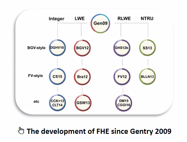
Figure 13: Development of Gentry’s Work as of 2020
Mechanism Behind HE
What objects support addition and multiplication? polynomials, matrices, and integers.
Today we use [GHDV09] as an example, which may seems a bit untidy, but still good enough to demonstrate the basic ideas of HE.
The construction of [GHDV09]:
- Secret Key
- large odd prime \(p\)
Encrypt a bit \(b\) - Pick a random large multiple of \(p\), \(q \cdot p\) - Pick a small \(r\) and let cipher text be \(c=q\cdot p+2r+b\)
- Decrypt a ciphertext \(c\)
- first \(\mod p\) then \(\mod 2\)
The noise is added to prevent GCD attacks in the IND-CPA game: GCD(\(p \cdot q_1\), \(p \cdot q_2\)) = \(p\). We rely on an “approximate-GCD” assumption.
When we perform homomorphic multiplication, there will be a quadratic blow-up in noise. When the noise grows too big, and becomes bigger than \(\frac{p}{2}\) then decryption security will be violated.
Now we can do a lot of additions and some multiplications. We have a “somewhat” homomorphic scheme. Enough to perform some low-multiplicative-depth tasks, like database search, spam filtering, etc.
The last step is accomplished through bootstrapping.
From Somewhat HE to Full HE
Consider an “augmented decryption circuit”
First decrypt \(c_1\) and \(c_2\) and them perform an NAND. We call this circuit \(\hat{C}\). The first layer of circuit \(\hat{C}\) has input \(c_1\) (resp. \(c_2\)) and \(sk\). If \(\hat{C}\) is in the evaluatable range of SHE, then Gentry shows that this SHE scheme actually implies a FHE scheme.
The natural idea is that decryption will kill all noise, so we can use decryption circuit to reduce all noise. Only the secret key are encryption, since the ciphertext is already public. So the output only carries noise from encryption of secret key, which is fresh every time. To summarize, we thus have obtained a “refresh” operation.
Issues Omitted
- The SWHE cannot correctly evaluate its decryption circuit, we have to “squash” this circuit by leaking some information of decryption key
- Is it safe to encrypt the key by itself? The circular security assumption still seems not proven to this day. In this example its self-loop.
- How to better control the noise accumulation? There are new scheme like GSW.
- Is it practical? NO.
FHE from LWE
LWE
Parameters: modulus \(q\), dimension \(n\), number of samples \(m\) Secret: uniformly random vector \(s \in \mathbb{Z}^n_q\). Noise: \(e\) sampled from some distribution such that \(|e| \ll q\) whp
Construction
- Public key
- \(A, b = As + 2e\), notice that here the multiple \(2\) is fine, since GCD(2, q) = 1, and we can reduce plain LWE to this version of “2LWE” by multiplying \(2^{-1}\) on both sides.
- Encryption
- Sample \(t \leftarrow \{0,1\}^m\) and \(c = t A, t b + m\).
Homomorphic Addition
Adding two ciphertexts together, also, since the modulus is \(q\), the ciphertext will not expand every time.
Homomorphic Multiplication
If \(|e_1| \ll q\) and \(|e_2| \ll q\) then \(m_1\cdot m_2 = (2e_1 + m_1)(2e_2 + m_2) \mod q \mod 2\).
Then let \(a^{\prime} = t A\), \(e^{\prime} te \), we have
\begin{align*} m_1 \cdot m_2 &= (2e_1 + m_1) (2e_2 + m_2) \\ &= (b_1 - s^T a_1) (b_2 - s^T a_2) \end{align*}
So we have to provide quadratic terms of \(s_i s_j\) and 1-degree term \(s_i\) in encrypted form. But there is also a problem of coefficient of \(Enc(s_i)\), \(Enc(s_i\cdot s_j)\) too big. We then apply the binary representation trick, i.e. publish encryption of \(2^0s_i\), \(2^1s_i\), \(2^2 s_i\), \(\ldots\).
Issues Omitted
If we do not want to rely on circular security, we have to resort to limited multipliation depth, and the key length will be linear to the depth.
[BV14] presented some better noise management tricks, using a “sequentialization” technique.
Secure Computation
In this chapter we discuss secure multiparty computation.
First we construct an OT scheme based on PKE with obviously sampleable PKs. This property requires that
- A sampling algorithm can sample pk identically distributed to the pk in real \(KeyGen\) algorithm
- The sampled pk cannot have a decryption key.